
2. Solving Equations by Fixed Point Iteration (of Contraction Mappings)
References:
Section 1.2 of Sauer
Section 2.2 of Burden&Faires
2.1. Introduction
in the next section we will meet Newton’s Method for root-finding, which you might have seen in a calculus course. This is one very important example of a more genetal strategy of fixed-point iteration, so we start with that.
# We will often need resources from the modules numpy and pyplot:
import numpy as np
from matplotlib import pyplot as plt

# We can also import items from a module individually, so they can be used by "first name only".
# Here this is done for mathematical functions; in some later sections it will be done for all imports.
from numpy import cos
2.2. Fixed-point equations
A variant of stating equations as root-finding (\(f(x) = 0\)) is fixed-point form: given a function \(g:\mathbb{R} \to \mathbb{R}\) or \(g:\mathbb{C} \to \mathbb{C}\) (or even \(g:\mathbb{R}^n \to \mathbb{R}^n\); a later topic), find a fixed point of \(g\). That is, a value \(p\) for its argument such that
Such problems are interchangeable with root-finding. One way to convert from \(f(x) = 0\) to \(g(x) = x\) is defining
for any “weight function” \(w(x)\).
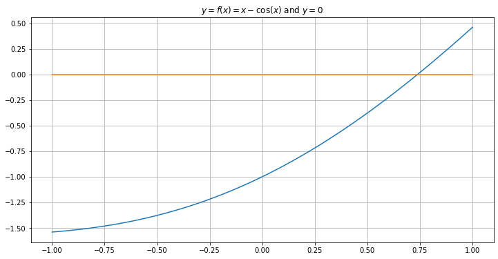
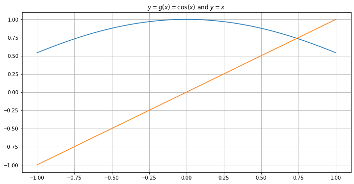
One can convert the other way too, for example defining \(f(x) := g(x) - x\). We have already seen this when we converted the equation \(x = \cos x\) to \(f(x) = x - \cos x = 0\).
Compare the two setups graphically: in each case, the \(x\) value at the intersection of the two curves is the solution we seek.
def f_1(x): return x - cos(x)
def g_1(x): return cos(x)
f = f_1
g = g_1
a = -1
b = 1

x = np.linspace(a, b)

plt.figure(figsize=(12,6))
plt.title('$y = f(x) = x - \cos(x)$ and $y=0$')
plt.plot(x, f(x))
plt.plot([a, b], [0, 0])
plt.grid(True)

plt.figure(figsize=(12,6))
plt.title('$y = g(x) = \cos (x)$ and $y=x$')
plt.plot(x, g(x))
plt.plot(x, x)
plt.grid(True)
The fixed point form can be convenient partly because we almost always have to solve by successive approximations, or iteration, and fixed point form suggests one choice of iterative procedure: start with any first approximation \(x_0\), and iterate with
Proposition 1. If \(g\) is continuous, and if the above sequence \(\{x_0, x_1, \dots \}\) converges to a limit \(p\), then that limit is a fixed point of function \(g\): \(g(p) = p\).
Proof: From \(\displaystyle \lim_{k \to \infty} x_k = p\), continuity gives
On the other hand, \(g(x_k) = x_{k+1}\), so
Comparing gives \(g(p) = p\).
That second “if” is a big one. Fortunately, it can often be resolved using the idea of a contraction mapping.
Definiton 1: Mapping. A function \(g(x)\) defined on a closed interval \(D = [a, b]\) which sends values back into that interval, \(g: D \to D\), is sometimes called a map or mapping.
(Aside: The same applies for a function \(g: D \to D\) where \(D\) is a subset of the complex numbers, or even of vectors \(\mathbb{R}^n\) or \(\mathbb{C}^n\).)
A mapping is sometimes thought of as moving a region \(S\) within its domain \(D\) to another such region, by moving each point \(x \in S \subset D\) to its image \(g(x) \in g(S) \subset D\).
A very important case is mappings that shrink the region, by reducing the distance between points:
Proposition 2: Any continuous mapping on a closed interval \([a, b]\) has at least one fixed point.
Proof: Consider the “root-finding cousin”, \(f(x) = x - g(x)\).
First, \(f(a) = a - g(a) \leq 0\), since \(g(a) \geq a\) so as to be in the domain \([a,b]\) — similarly, \(f(b) = b - g(b) \geq 0\).
From the Intermediate Value Theorem, \(f\) has a zero \(p\), where \(f(p) = p - g(p) = 0\).
In other words, the graph of \(y=g(x)\) goes from being above the line \(y=x\) at \(x=a\) to below it at \(x=b\), so at some point \(x=p\), the curves meet: \(y = x = p\) and \(y = g(p)\), so \(p = g(p)\).
2.2.1. Example 1
Let us illustrate this with the mapping \(g_4(x) := 4 \cos x\), for which the fact that \(|g_4(x)| \leq 4\) ensures that this is a map of the domain \(D = [-4, 4]\) into itself:
def g_4(x): return 4*cos(x)
a = -4
b = 4
x = np.linspace(a, b)

plt.figure(figsize=(12,6))
plt.title('Fixed points of the map $g_4(x) = 4 \cos(x)$')
plt.plot(x, g_4(x), label='$y=g_4(x)$')
plt.plot(x, x, label='$y=x$')
ignore_me = plt.legend()  # Note: the bogus output value "ignore_me" supresses some useless output
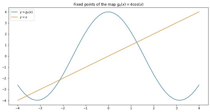
This example has multiple fixed points (three of them). To ensure both the existence of a unique solution, and covergence of the iteration to that solution, we need an extra condition.
Definition 2: Contraction Mapping. A mapping \(g:D \to D\), is called a contraction or contraction mapping if there is a constant \(C < 1\) such that
for any \(x\) and \(y\) in \(D\). We then call \(C\) a contraction constant.
(Aside: The same applies for a domain in \(\mathbb{R}^n\): just replace the absolute value \(| \dots |\) by the vector norm \(\| \dots \|\).)
Note: it is not enough to have \(| g(x) - g(y) | < | x - y |\) or \(C = 1\)! We need the ratio \(\displaystyle \frac{|g(x) - g(y)|}{|x - y|}\) to be uniformly less than one for all possible values of \(x\) and \(y\).
Theorem 1 (A Contraction Mapping Theorem). Any contraction mapping \(g\) on a closed, bounded interval \(D = [a, b]\) has exactly one fixed point \(p\) in \(D\). Further, this can be calculated as the limit \(\displaystyle p = \lim_{k \to \infty} x_k\) of the iteration sequence given by \(x_{k+1} = g(x_{k})\) for any choice of the starting point \(x_{0} \in D\).
Proof:
The main idea of the proof can be shown with the help of a few pictures.
First, uniqeness:
between any two of the multiple fixed points above — call them \(p_0\) and \(p_1\) — the graph of \(g(x)\) has to rise with secant slope 1: \((g(p_1) - g(p_0)/(p_1 - p_0) = (p_1 - p_0)/(p_1 - p_0) = 1\), and this violates the contraction property.
So instead, for a contraction, the graph of a contraction map looks like the one below for our favorite example, \(g(x) = \cos x\) (which we will soon verify to be a contraction on interval \([-1, 1]\)):
The second claim, about convergence to the fixed point from any initial approximation \(x_0\), will be verified below, once we have seen some ideas about measuring errors.
2.2.2. An easy way of checking whether a differentiable function is a contraction
With differentiable functions, the contraction condition can often be easily verified using derivatives:
Theorem 2 (A derivative-based fixed point theorem). If a function \(g:[a,b] \to [a,b]\) is differentiable and there is a constant \(C < 1\) such that \(|g'(x)| \leq C\) for all \(x \in [a, b]\), then \(g\) is a contraction mapping, and so has a unique fixed point in this interval.
Proof:
Using the Mean Value Theorem, \(g(x) - g(y) = g'(c)(x - y)\) for some \(c\) between \(x\) and \(y\);
then taking absolute values,
2.2.3. Example 2. \(g(x) = \cos x\) is a contraction on domain \([-1, 1]\)
Our favorite example \(g(x) = \cos(x)\) is a contraction, but we have to be a bit careful about the domain.
For all real \(x\), \(g'(x) = -\sin x\), so \(|g'(x)| \leq 1\); this is almost but not quite enough.
However, we have seen that iteration values will settle in the interval \(D = [-1,1]\), and considering \(g\) as a mapping of this domain, \(|g'(x)| \leq \sin(1) = 0.841\dots < 1\): that is, now we have a contraction, with \(C = \sin(1) \approx 0.841\).
And as seen in the graph above, there is indeed a unique fixed point.
2.2.4. The contraction constant \(C\) as a measure of how fast the approximations improve (the smaller the better)
It can be shown that if \(C\) is small (at least when one looks only at a reduced domain \(|x - p| < R\)) then the convergence is “fast” once \(|x_k - p| < R\).
To see this, we define some jargon for talking about errors. (For more details on error concepts, see the section on Measures of Error and Convergence Rates)
Definition 3: Error. The error in \(\tilde x\) as an approximation to an exact value \(x\) is
This will often be abbreviated as \(E\).
Definition 4: Absolute Error. The absolute error in \(\tilde x\) an approximation to an exact value \(x\) is the magnitude of the error: the absolute value \(|E| = |\tilde x - x|\).
(Aside: This will later be extended to \(x\) and \(\tilde x\) being vectors, by again using the vector norm in place of the absolute value. In fact, I will sometimes blur the distinction by using the “single line” absolute value notation for vector norms too.)
In the case of \(x_k\) as an approximation of \(p\), we name the error \(E_k := x_k - p\). Then \(C\) measures a worst case for how fast the error decreases as \(k\) increases, and this is “exponentially fast”:
Proposition 3. \(|E_{k+1}| \leq C |E_{k}|\), or \(|E_{k+1}|/|E_{k}|\leq C\), and so
That is, the error decreases at worst in a geometric sequence, which is exponential decrease with respect to the variable \(k\).
Proof.
\(E_{k+1} = x_{k+1} - p = g(x_{k}) - g(p)\), using \(g(p) = p\). Thus the contraction property gives
Applying this again,
and repeating \(k-2\) more times,
Aside: We will often use this “recursive” strategy of relating the error in one iterate to that in the previous iterate.
The rest of the proof of the Contraction Mapping Theorem (Theorem 5): guaranteed convergence.
This now follows from the above proposition:
for any initial approximation \(x_0\), we know that
\(|E_k|\leq C^k |x_0 - p|\), and with \(C < 1\), this can be made as small as we want by choosing a large enough value of \(k\).
Thus
which is another way of saying that \(\displaystyle \lim_{k \to \infty} x_k = p\), or \(x_k \to p\), as claimed.
2.2.5. Example 3. Solving \(x = \cos x\) with a naive fixed point iteration
We have seen that one way to convert the example \(f(x) = x - \cos x = 0\) to a fixed point iteration is \(g(x) = \cos x\), and that this is a contraction on \(D = [-1, 1]\)
Here is what this iteration looks like:
g = g_1
a = 0
b = 1
x = np.linspace(a, b)
iterations = 10

# Start at left
print(f"Solving x = cos(x) starting to the left, at x_0 = {a}")
x_k = a
plt.figure(figsize=(8,8))
plt.title(f"Solving $x = \cos x$ starting to the left, at $x_0$ = {a}")
plt.plot(x, x, 'g')
plt.plot(x, g(x), 'r')
for k in range(iterations):
    g_x_k = g(x_k)
    # Graph evalation of g(x_k) from x_k:
    plt.plot([x_k, x_k], [x_k, g(x_k)], 'b')
    x_k_plus_1 = g(x_k)
    #Connect to the new x_k on the line y = x:
    plt.plot([x_k, g(x_k)], [x_k_plus_1, x_k_plus_1], 'b')
    # Update names: the old x_k+1 is the new x_k
    x_k = x_k_plus_1
    print(f"x_{k+1} = {x_k_plus_1}")

plt.show()

# Start at right
print(f"Solving x = cos(x) starting to the right, at x_0 = {b}")
x_k = b
plt.figure(figsize=(8,8))
plt.title(f"Solving $x = \cos(x)$ starting to the right, at $x_0$ = {b}")
plt.plot(x, x, 'g')
plt.plot(x, g(x), 'r')
for k in range(iterations):
    g_x_k = g(x_k)
    # Graph evalation of g(x_k) from x_k:
    plt.plot([x_k, x_k], [x_k, g(x_k)], 'b')
    x_k_plus_1 = g(x_k)
    #Connect to the new x_k on the line y = x:
    plt.plot([x_k, g(x_k)], [x_k_plus_1, x_k_plus_1], 'b')
    # Update names: the old x_k+1 is the new x_k
    x_k = x_k_plus_1
    print(f"x_{k+1} = {x_k_plus_1}")
Solving x = cos(x) starting to the left, at x_0 = 0
x_1 = 1.0
x_2 = 0.5403023058681398
x_3 = 0.8575532158463934
x_4 = 0.6542897904977791
x_5 = 0.7934803587425656
x_6 = 0.7013687736227565
x_7 = 0.7639596829006542
x_8 = 0.7221024250267079
x_9 = 0.7504177617637604
x_10 = 0.7314040424225099

Solving x = cos(x) starting to the right, at x_0 = 1
x_1 = 0.5403023058681398
x_2 = 0.8575532158463934
x_3 = 0.6542897904977791
x_4 = 0.7934803587425656
x_5 = 0.7013687736227565
x_6 = 0.7639596829006542
x_7 = 0.7221024250267079
x_8 = 0.7504177617637604
x_9 = 0.7314040424225099
x_10 = 0.7442373549005569
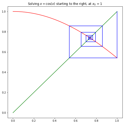
In each case, one gets a “box spiral” in to the fixed point. It always looks like this when \(g\) is decreasing near the fixed point.
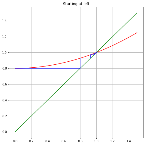
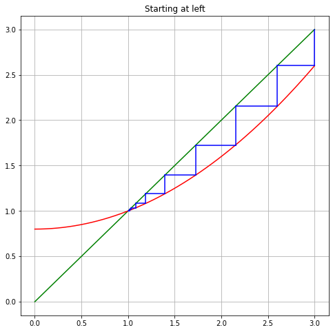
If instead \(g\) is increasing near the fixed point, the iterates approach monotonically, either from above or below:
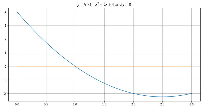
2.2.6. Example 4. Solving \(f(x) = x^2 - 5x + 4 = 0\) in interval \([0, 3]\)
The roots are 1 and 4; for now we aim at the first of these, so we chose a domain \([0, 3]\) that contains just this root.
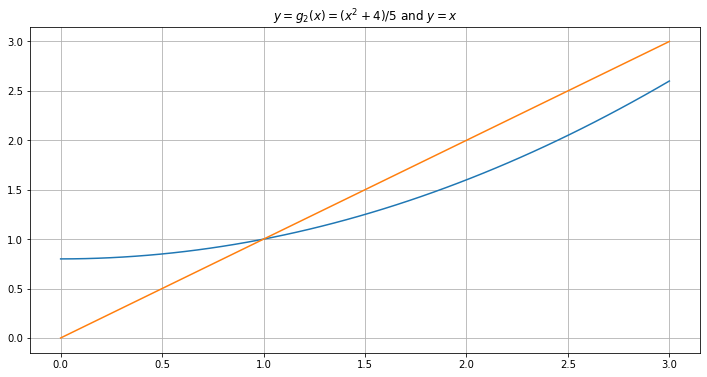
Let us get a fixed point for by “partially solving for \(x\)”: solving for the \(x\) in the \(5 x\) term:
def f_2(x): return x**2 - 5*x + 4
def g_2(x): return (x**2 + 4)/5
f = f_2
g = g_2
a = 0
b = 3
x = np.linspace(a, b)

plt.figure(figsize=(12,6))
plt.title('$y = f_2(x) = x^2-5x+4$ and $y = 0$')
plt.plot(x, f(x))
plt.plot([a, b], [0, 0])
plt.grid(True)

plt.figure(figsize=(12,6))
plt.title('$y = g_2(x) = (x^2 + 4)/5$ and $y=x$')
plt.plot(x, g(x))
plt.plot(x, x)
plt.grid(True)
iterations = 10
g = g_2
# Start at left
a = 0
b = 1.5
x = np.linspace(a, b)
print(f"Starting to the left, at x_0 = {a}")
x_k = a
plt.figure(figsize=(8,8))
plt.title('Starting at left')
plt.grid(True)
plt.plot(x, x, 'g')
plt.plot(x, g(x), 'r')
for k in range(iterations):
    g_x_k = g(x_k)
    # Graph evalation of g(x_k) from x_k:
    plt.plot([x_k, x_k], [x_k, g(x_k)], 'b')
    x_k_plus_1 = g(x_k)
    #Connect to the new x_k on the line y = x:
    plt.plot([x_k, g_2(x_k)], [x_k_plus_1, x_k_plus_1], 'b')
    # Update names: the old x_k+1 is the new x_k
    x_k = x_k_plus_1
    print(f"x_{k+1} = {x_k_plus_1}")

plt.show()

# Start at right
a = 0
b = 3
x = np.linspace(a, b)
print(f"Starting to the right, at x_0 = {b}")
x_k = b
plt.figure(figsize=(8,8))
plt.title('Starting at left')
plt.grid(True)
plt.plot(x, x, 'g')
plt.plot(x, g(x), 'r')
for k in range(iterations):
    g_x_k = g(x_k)
    # Graph evalation of g(x_k) from x_k:
    plt.plot([x_k, x_k], [x_k, g(x_k)], 'b')
    x_k_plus_1 = g(x_k)
    #Connect to the new x_k on the line y = x:
    plt.plot([x_k, g(x_k)], [x_k_plus_1, x_k_plus_1], 'b')
    # Update names: the old x_k+1 is the new x_k
    x_k = x_k_plus_1
    print(f"x_{k+1} = {x_k_plus_1}")
Starting to the left, at x_0 = 0
x_1 = 0.8
x_2 = 0.9280000000000002
x_3 = 0.9722368000000001
x_4 = 0.9890488790548482
x_5 = 0.9956435370319303
x_6 = 0.9982612105666906
x_7 = 0.9993050889044148
x_8 = 0.999722132142052
x_9 = 0.9998888682989302
x_10 = 0.999955549789623
Starting to the right, at x_0 = 3
x_1 = 2.6
x_2 = 2.152
x_3 = 1.7262208
x_4 = 1.3959676500705283
x_5 = 1.1897451360086866
x_6 = 1.0830986977312658
x_7 = 1.0346205578054328
x_8 = 1.014087939726725
x_9 = 1.0056748698998388
x_10 = 1.0022763887896116
This work is licensed under Creative Commons Attribution-ShareAlike 4.0 International