
Notebook for generating the module numerical_methods_module
Author: Brenton LeMesurier, brenton.lemesurier@unco.edu and lemesurierb@cofc.edu
A collection of functions implementing numerical algorithms from the course and book Elementary Numerical Analysis,
and a module numerical_methods_module produced from that.
Last updated on April 11, 2021
Recent additions; most recent first:
a function
inversefor computing the inverse of a matrix (but use this sparingly!)versions of Euler’s Method and the Classical Runge-Kutta Method for systems.
Zero Finding: solving \(f(x) = 0\) or \(g(x) = x\)
def bisection1(f, a, b, N, demoMode=False):
    '''Approximately solve equation f(x) = 0 in the interval [a, b] with N iterations of the Bisection Method.
    By the way, a triple-quoted multi-line comment like this provides covenient documentation about what a function does,
    so I encourage adding them. Try the commmand `help(bisection1)`
    '''
    c = (a + b)/2
    for iteration in range(N):
        if demoMode: print(f"\nIteration {iteration+1}:")
        if f(a) * f(c) < 0:
            b = c
        else:
            a = c
        c = (a + b)/2
        if demoMode:
            print(f"The root is in interval [{a}, {b}]")
            print(f"The new approximation is {c}, with backward error {np.abs(f(c)):0.3}")
        root = c
        errorBound = (c-a)
    return (c, errorBound)
# Demo
if __name__ == "__main__":  # Do this if running the .py file directly, but not when importing [from] it
    def f(x): return x - np.cos(x)
    print("Solving by the Bisection Method.")
    (root, errorBound) = bisection1(f, a=-1, b=1, N=10, demoMode=True)
    print(f"\n{root=}, backward error {np.abs(f(root)):0.3}")
Solving by the Bisection Method.

Iteration 1:
The root is in interval [0.0, 1]
The new approximation is 0.5, with backward error 0.378

Iteration 2:
The root is in interval [0.5, 1]
The new approximation is 0.75, with backward error 0.0183

Iteration 3:
The root is in interval [0.5, 0.75]
The new approximation is 0.625, with backward error 0.186

Iteration 4:
The root is in interval [0.625, 0.75]
The new approximation is 0.6875, with backward error 0.0853

Iteration 5:
The root is in interval [0.6875, 0.75]
The new approximation is 0.71875, with backward error 0.0339

Iteration 6:
The root is in interval [0.71875, 0.75]
The new approximation is 0.734375, with backward error 0.00787

Iteration 7:
The root is in interval [0.734375, 0.75]
The new approximation is 0.7421875, with backward error 0.0052

Iteration 8:
The root is in interval [0.734375, 0.7421875]
The new approximation is 0.73828125, with backward error 0.00135

Iteration 9:
The root is in interval [0.73828125, 0.7421875]
The new approximation is 0.740234375, with backward error 0.00192

Iteration 10:
The root is in interval [0.73828125, 0.740234375]
The new approximation is 0.7392578125, with backward error 0.000289

root=0.7392578125, backward error 0.000289
def fpi(g, x_0, errorTolerance=1e-6, maxIterations=20, demoMode=False):
    """Fixed point iteration for approximately solving x = f(x),
    x_0: the initial value
    """
    x = x_0
    for iteration in range(maxIterations):
        x_new = g(x)
        errorEstimate = np.abs(x_new - x)
        x = x_new
        if demoMode: print(f"x_{iteration} = {x}, {errorEstimate=:0.3}")
        if errorEstimate <= errorTolerance: break
    return (x, errorEstimate)
# Demo
if __name__ == "__main__":  # Do this if running the .py file directly, but not when importing [from] it
    def g(x): return np.cos(x)
    print("Fixed point iteration.")
    (root, errorEstimate) = fpi(g, 0, demoMode=True)
    print(f"\n{root=}, {errorEstimate=}")
Fixed point iteration.
x_0 = 1.0, errorEstimate=1.0
x_1 = 0.5403023058681398, errorEstimate=0.46
x_2 = 0.8575532158463934, errorEstimate=0.317
x_3 = 0.6542897904977791, errorEstimate=0.203
x_4 = 0.7934803587425656, errorEstimate=0.139
x_5 = 0.7013687736227565, errorEstimate=0.0921
x_6 = 0.7639596829006542, errorEstimate=0.0626
x_7 = 0.7221024250267079, errorEstimate=0.0419
x_8 = 0.7504177617637604, errorEstimate=0.0283
x_9 = 0.7314040424225099, errorEstimate=0.019
x_10 = 0.7442373549005569, errorEstimate=0.0128
x_11 = 0.7356047404363473, errorEstimate=0.00863
x_12 = 0.7414250866101093, errorEstimate=0.00582
x_13 = 0.7375068905132427, errorEstimate=0.00392
x_14 = 0.7401473355678758, errorEstimate=0.00264
x_15 = 0.7383692041223231, errorEstimate=0.00178
x_16 = 0.7395672022122561, errorEstimate=0.0012
x_17 = 0.7387603198742112, errorEstimate=0.000807
x_18 = 0.739303892396906, errorEstimate=0.000544
x_19 = 0.7389377567153443, errorEstimate=0.000366

root=0.7389377567153443, errorEstimate=0.0003661356815616301
def newton(f, Df, x0, errorTolerance=1e-15, maxIterations=20, demoMode=False):
    """Basic usage is:
    (rootApproximation, errorEstimate, iterations) = newton(f, Df, x0, errorTolerance)
    There is an optional input parameter "demoMode" which controls whether to
    - print intermediate results (for "study" purposes), or to
    - work silently (for "production" use).
    The default is silence.

    """
    x = x0
    for k in range(1, maxIterations+1):
        fx = f(x)
        Dfx = Df(x)
        # Note: a careful, robust code would check for the possibility of division by zero here,
        # but for now I just want a simple presentation of the basic mathematical idea.
        dx = fx/Dfx
        x -= dx  # Aside: this is shorthand for "x = x - dx"
        errorEstimate = abs(dx)
        if demoMode:
            print(f"At iteration {k} x = {x} with estimated error {errorEstimate:0.3}, backward error {abs(f(x)):0.3}")
        if errorEstimate <= errorTolerance:
            iterations = k
            return (x, errorEstimate, iterations)
    # If we get here, it did not achieve the accuracy target:
    iterations = k
    return (x, errorEstimate, iterations)
# Demo
if __name__ == "__main__":  # Do this if running the .py file directly, but not when importing [from] it
    def f(x): return x - np.cos(x)
    def Df(x): return 1. + np.sin(x)
    print("Solving by Newton's Method.")
    (root, errorEstimate, iterations) = newton(f, Df, x0=0.,
                                               errorTolerance=1e-8, demoMode=True)
    print()
    print(f"The root is approximately {root}")
    print(f"The estimated absolute error is {errorEstimate}")
    print(f"The backward error is {abs(f(root)):0.3}")
    print(f"This required {iterations} iterations")
Solving by Newton's Method.
At iteration 1 x = 1.0 with estimated error 1.0, backward error 0.46
At iteration 2 x = 0.7503638678402439 with estimated error 0.25, backward error 0.0189
At iteration 3 x = 0.7391128909113617 with estimated error 0.0113, backward error 4.65e-05
At iteration 4 x = 0.7390851333852839 with estimated error 2.78e-05, backward error 2.85e-10
At iteration 5 x = 0.7390851332151606 with estimated error 1.7e-10, backward error 1.11e-16

The root is approximately 0.7390851332151606
The estimated absolute error is 1.7012334067709158e-10
The backward error is 1.11e-16
This required 5 iterations
def false_position(f, a, b, errorTolerance=1e-15, maxIterations=15, demoMode=False):
    """Solve f(x)=0 in the interval [a, b] by the Method of False Position.
    This code also illustrates a few ideas that I encourage, such as:
    - Avoiding infinite loops, by using for loops sand break
    - Avoiding repeated evaluation of the same quantity
    - Use of descriptive variable names
    - Use of "camelCase" to turn descriptive phrases into valid Python variable names
    - An optional "demonstration mode" to display intermediate results.
    """
    fa = f(a)
    fb = f(b)
    for iteration in range(1, maxIterations+1):
        if demoMode: print(f"\nIteration {iteration}:")
        c = (a * fb - fa * b)/(fb - fa)
        fc = f(c)
        if fa * fc < 0:
            b = c
            fb = fc  # N.B. When b is updated, so must be fb = f(b)
        else:
            a = c
            fa = fc
        errorBound = b - a
        if demoMode:
            print(f"The root is in interval [{a}, {b}]")
            print(f"The new approximation is {c}, with error bound {errorBound:0.3}, backward error {abs(fc):0.3}")
        if errorBound < errorTolerance:
            break
    # Whether we got here due to accuracy of running out of iterations,
    # return the information we have, including an error bound:
    root = c  # the newest value is probably the most accurate
    return (root, errorBound)
# Demo
if __name__ == "__main__":  # Do this if running the .py file directly, but not when importing [from] it
    def f(x): return x - np.cos(x)
    print("Solving by the Method of False Position.")
    (root, errorBound) = false_position(f, a=-1, b=1, demoMode=True)
    print(f"\nThe Method of False Position gave approximate root is {root},")
    print(f"with estimate error {errorBound:0.3}, backward error {abs(f(root)):0.3}")
Solving by the Method of False Position.

Iteration 1:
The root is in interval [0.5403023058681398, 1]
The new approximation is 0.5403023058681398, with error bound 0.46, backward error 0.317

Iteration 2:
The root is in interval [0.7280103614676172, 1]
The new approximation is 0.7280103614676172, with error bound 0.272, backward error 0.0185

Iteration 3:
The root is in interval [0.7385270062423998, 1]
The new approximation is 0.7385270062423998, with error bound 0.261, backward error 0.000934

Iteration 4:
The root is in interval [0.7390571666782676, 1]
The new approximation is 0.7390571666782676, with error bound 0.261, backward error 4.68e-05

Iteration 5:
The root is in interval [0.7390837322783136, 1]
The new approximation is 0.7390837322783136, with error bound 0.261, backward error 2.34e-06

Iteration 6:
The root is in interval [0.7390850630385933, 1]
The new approximation is 0.7390850630385933, with error bound 0.261, backward error 1.17e-07

Iteration 7:
The root is in interval [0.7390851296998365, 1]
The new approximation is 0.7390851296998365, with error bound 0.261, backward error 5.88e-09

Iteration 8:
The root is in interval [0.7390851330390691, 1]
The new approximation is 0.7390851330390691, with error bound 0.261, backward error 2.95e-10

Iteration 9:
The root is in interval [0.7390851332063397, 1]
The new approximation is 0.7390851332063397, with error bound 0.261, backward error 1.48e-11

Iteration 10:
The root is in interval [0.7390851332147188, 1]
The new approximation is 0.7390851332147188, with error bound 0.261, backward error 7.39e-13

Iteration 11:
The root is in interval [0.7390851332151385, 1]
The new approximation is 0.7390851332151385, with error bound 0.261, backward error 3.71e-14

Iteration 12:
The root is in interval [0.7390851332151596, 1]
The new approximation is 0.7390851332151596, with error bound 0.261, backward error 1.78e-15

Iteration 13:
The root is in interval [0.7390851332151606, 1]
The new approximation is 0.7390851332151606, with error bound 0.261, backward error 1.11e-16

Iteration 14:
The root is in interval [0.7390851332151607, 1]
The new approximation is 0.7390851332151607, with error bound 0.261, backward error 0.0

Iteration 15:
The root is in interval [0.7390851332151607, 1]
The new approximation is 0.7390851332151607, with error bound 0.261, backward error 0.0

The Method of False Position gave approximate root is 0.7390851332151607,
with estimate error 0.261, backward error 0.0
def secant_method(f, a, b, errorTolerance=1e-15, maxIterations=15, demoMode=False):
    """Solve f(x)=0 in the interval [a, b] by the Secant Method."""
    # Some more descriptive names
    x_older = a
    x_more_recent = b
    f_x_older = f(x_older)
    f_x_more_recent = f(x_more_recent)
    for iteration in range(1, maxIterations+1):
        if demoMode: print(f"\nIteration {iteration}:")
        x_new = (x_older * f_x_more_recent - f_x_older * x_more_recent)/(f_x_more_recent - f_x_older)
        f_x_new = f(x_new)
        (x_older, x_more_recent) = (x_more_recent, x_new)
        (f_x_older, f_x_more_recent) = (f_x_more_recent, f_x_new)
        errorEstimate = abs(x_older - x_more_recent)
        if demoMode:
            print(f"The latest pair of approximations are {x_older} and {x_more_recent},")
            print(f"where the function's values are {f_x_older:0.3} and {f_x_more_recent:0.3} respectively.")
            print(f"The new approximation is {x_new}, with estimated error {errorEstimate:0.3}, backward error {abs(f_x_new):0.3}")
        if errorEstimate < errorTolerance:
            break
    # Whether we got here due to accuracy of running out of iterations,
    # return the information we have, including an error estimate:
    return (x_new, errorEstimate)
# Demo
if __name__ == "__main__":  # Do this if running the .py file directly, but not when importing [from] it
    def f(x): return x - np.cos(x)
    print(f"Solving by the Secant Method.")
    (root, errorEstimate) = secant_method(f, a=-1, b=1, demoMode=True)
    print(f"\nThe Secant Method gave approximate root is {root},")
    print(f"with estimated error {errorEstimate:0.3}, backward error {abs(f(root)):0.3}")
Solving by the Secant Method.

Iteration 1:
The latest pair of approximations are 1 and 0.5403023058681398,
where the function's values are 0.46 and -0.317 respectively.
The new approximation is 0.5403023058681398, with estimated error 0.46, backward error 0.317

Iteration 2:
The latest pair of approximations are 0.5403023058681398 and 0.7280103614676172,
where the function's values are -0.317 and -0.0185 respectively.
The new approximation is 0.7280103614676172, with estimated error 0.188, backward error 0.0185

Iteration 3:
The latest pair of approximations are 0.7280103614676172 and 0.7396270126307336,
where the function's values are -0.0185 and 0.000907 respectively.
The new approximation is 0.7396270126307336, with estimated error 0.0116, backward error 0.000907

Iteration 4:
The latest pair of approximations are 0.7396270126307336 and 0.7390838007832722,
where the function's values are 0.000907 and -2.23e-06 respectively.
The new approximation is 0.7390838007832722, with estimated error 0.000543, backward error 2.23e-06

Iteration 5:
The latest pair of approximations are 0.7390838007832722 and 0.7390851330557805,
where the function's values are -2.23e-06 and -2.67e-10 respectively.
The new approximation is 0.7390851330557805, with estimated error 1.33e-06, backward error 2.67e-10

Iteration 6:
The latest pair of approximations are 0.7390851330557805 and 0.7390851332151607,
where the function's values are -2.67e-10 and 0.0 respectively.
The new approximation is 0.7390851332151607, with estimated error 1.59e-10, backward error 0.0

Iteration 7:
The latest pair of approximations are 0.7390851332151607 and 0.7390851332151607,
where the function's values are 0.0 and 0.0 respectively.
The new approximation is 0.7390851332151607, with estimated error 0.0, backward error 0.0

The Secant Method gave approximate root is 0.7390851332151607,
with estimated error 0.0, backward error 0.0
Linear Algebra
Basic row reduction elimination and backward substitution
def rowReduce(A, b):
    """To avoid modifying the matrix and vector specified as input,
    they are copyied to new arrays, with the method .copy()
    Warning: it does not work to say "U = A" and "c = b";
    this makes these names synonyms, referring to the same stored data.
    Also: this doe not modify the vlaue of U belwo th main diagonal,
    since they are know to be zero, an wil bever be used;
    to clean this up, use function zeros_below_diagonal.
    """
    U = A.copy()
    c = b.copy()
    n = len(b)
    # The function zeros_like() is used to create L with the same size and shape as A,
    # and with all its elements zero initially.
    L = np.zeros_like(A)
    for k in range(n-1):
        for i in range(k+1, n):
            L[i,k] = U[i,k] / U[k,k]
            for j in range(k+1, n):
                U[i,j] = U[i,j] - L[i,k] * U[k,j]
            c[i]= c[i] - L[i,k] * c[k]
    return (U, c)
Immediately updated to the following, but I leave the first version for reference.
def rowReduce(A, b):
    """To avoid modifying the matrix and vector specified as input,
    they are copied to new arrays, with the method .copy()
    Warning: it does not work to say "U = A" and "c = b";
    this makes these names synonyms, referring to the same stored data.
    This code leaves "garbage values" below the main diagonal
    if needed, clean up with the function zeros_below_diagonal.
    """
    U = A.copy()
    c = b.copy()
    n = len(b)
    # The function zeros_like() is used to create L with the same size and shape as A,
    # and with all its elements zero initially.
    L = np.zeros_like(A)
    for k in range(n-1):
        # compute all the L values for column k:
        L[k+1:n,k] = U[k+1:n,k] / U[k,k]  # Beware the case where U[k,k] is 0
        for i in range(k+1, n):
            U[i,k+1:n] -= L[i,k] * U[k,k+1:n]  # Update row i
        c[k+1:n] -= L[k+1:n,k] * c[k]  # update c values
    return (U, c)
Further updated on March 7 as follows, adding demoMode and “zeroing” below the main diagonal in U when using that mode.
def rowReduce(A, b, demoMode=False):
    """To avoid modifying the matrix and vector specified as input,
    they are copied to new arrays, with the method .copy()
    Warning: it does not work to say "U = A" and "c = b";
    this makes these names synonyms, referring to the same stored data.
    This code leaves "garbage values" below the main diagonal
    if needed, clean up with the function zeros_below_diagonal.

    2021-03-07: added a demonstration mode.
    """
    U = A.copy()
    c = b.copy()
    n = len(b)
    # The function zeros_like() is used to create L with the same size and shape as A,
    # and with all its elements zero initially.
    L = np.zeros_like(A)
    for k in range(n-1):
        if demoMode: print(f"Step {k=}")
        # compute all the L values for column k:
        L[k+1:,k] = U[k+1:n,k] / U[k,k]  # Beware the case where U[k,k] is 0
        if demoMode:
            print(f"The multipliers in column {k+1} are {L[k+1:,k]}")
        for i in range(k+1, n):
            U[i,k+1:n] -= L[i,k] * U[k,k+1:n]  # Update row i
        c[k+1:n] -= L[k+1:n,k] * c[k]  # update c values
        if demoMode:
            # insert zeros in U:
            U[k+1:, k] = 0.
            print(f"The updated matrix is\n{U}")
            print(f"The updated right-hand side is\n{c}")
    return (U, c)
def zeros_below_diagonal(U):
    """Insert the below-diagonal zero values into U, ignored in function rowReduce.
    These are needed to display U correctly,
    and to demonstrate that the new system of equations Ux=c has the same solution as Ax=b.
    """
    for i in range(1,len(U)):
        for j in range(i):
            U[i,j] = 0.
As with rowReduce, this is immediately updated to the following, but I leave the first version for reference.
def zeros_below_diagonal(U):
    """Insert the below-diagonal zero values into U, ignored in the function rowReduce.
    These are needed to display U correctly,
    and to demonstrate that the new system of equations Ux=c$ has the same solution as Ax=b.
    """
    for i in range(1,len(U)):
        U[i,:i] = 0.
# Demo
if __name__ == "__main__":  # Do this if running the .py file directly, but not when importing [from] it
#    A = np.array([[4. , 235. , 7.], [3. , 5. , -6.],[1. , -3. , 22.]])
    A = np.array([[1. , -3. , 15.], [5. , 200. , 7.], [4. , 11. , -6.]])
    print(f"A =\n{A}")
#    b = np.array([2. , 3. , 4.])
    b = np.array([4. , 3. , 2.])
    print(f"b = {b}")

    (U, c) = rowReduce(A, b, demoMode=True)
    zeros_below_diagonal(U)
    print(f"U =\n{U}")
    print(f"c = {c}")
A =
[[  1.  -3.  15.]
 [  5. 200.   7.]
 [  4.  11.  -6.]]
b = [4. 3. 2.]
Step k=0
The multipliers in column 1 are [5. 4.]
The updated matrix is
[[  1.  -3.  15.]
 [  0. 215. -68.]
 [  0.  23. -66.]]
The updated right-hand side is
[  4. -17. -14.]
Step k=1
The multipliers in column 2 are [0.10697674]
The updated matrix is
[[  1.         -3.         15.       ]
 [  0.        215.        -68.       ]
 [  0.          0.        -58.7255814]]
The updated right-hand side is
[  4.         -17.         -12.18139535]
U =
[[  1.         -3.         15.       ]
 [  0.        215.        -68.       ]
 [  0.          0.        -58.7255814]]
c = [  4.         -17.         -12.18139535]
def backwardSubstitution(U, c):
    """Solve U x = c for b."""
    n = len(c)
    x = np.zeros(n)
    x[-1] = c[-1]/U[-1,-1]
    for i in range(2, n+1):
        x[-i] = (c[-i] - sum(U[-i,1-i:] * x[1-i:])) / U[-i,-i]
    return x
UPDATE: this was further updated on March 7 as follows, mainly to add demoMode.
def backwardSubstitution(U, c, demoMode=False):
    """Solve U x = c for b.

    2021-03-07: aded a demonstration mode.
    """
    n = len(c)
    x = np.zeros(n)
    x[-1] = c[-1]/U[-1,-1]
    if demoMode: print(f"x_{n} = {x[-1]}")
    for i in range(2, n+1):
        x[-i] = (c[-i] - sum(U[-i,1-i:] * x[1-i:])) / U[-i,-i]
        if demoMode: print(f"x_{n-i+1} = {x[-i]}")
    return x
# Demo
if __name__ == "__main__":  # Do this if running the .py file directly, but not when importing [from] it
    x = backwardSubstitution(U, c, demoMode=True)
    print("")
    print(f"x = {x}")
    r = b - A@x
    print(f"The residual b - Ax = {r},")
    print(f"with maximum norm {max(abs(r)):.3}.")
x_3 = 0.20742911452558213
x_2 = -0.013464280057025185
x_1 = 0.8481704419451925

x = [ 0.84817044 -0.01346428  0.20742911]
The residual b - Ax = [ 0.0000000e+00 -8.8817842e-16 -4.4408921e-16],
with maximum norm 8.88e-16.
LU factorization …
def lu(A, demoMode=False):
    """Compute the Doolittle LU factorization of A.
    Sums like $\sum_{s=1}^{k-1} l_{k,s} u_{s,j}$ are done as matrix products;
    in the above case, row matrix L[k, 1:k-1] by column matrix U[1:k-1,j] gives the sum for a give j,
    and row matrix L[k, 1:k-1] by matrix U[1:k-1,k:n] gives the relevant row vector.
    """
    n = len(A)  # len() gives the number of rows in a 2D array.
    # Initialize U as the zero matrix;
    # correct below the main diagonal, with the other entries to be computed below.
    U = np.zeros_like(A)
    # Initialize L as the identity matrix;
    # correct on and above the main diagonal, with the other entries to be computed below.
    L = np.identity(n)
   # Column and row 1 (i.e Python index 0) are special:
    U[0,:] = A[0,:]
    L[1:,0] = A[1:,0]/U[0,0]
    if demoMode:
        print(f"After step k=0")
        print(f"U=\n{U}")
        print(f"L=\n{L}")
    for k in range(1, n-1):
        U[k,k:] = A[k,k:] - L[k,:k] @ U[:k,k:]
        L[k+1:,k] = (A[k+1:,k] - L[k+1:,:k] @ U[:k,k])/U[k,k]
        if demoMode:
            print(f"After step {k=}")
            print(f"U=\n{U}")
            print(f"L=\n{L}")
    # The last row (index "-1") is special: nothing to do for L
    U[-1,-1] = A[-1,-1] - sum(L[-1,:-1]*U[:-1,-1])
    if demoMode:
        print(f"After the final step, k={n-1}")
        print(f"U=\n{U}")
    return (L, U)
# Demo
if __name__ == "__main__":  # Do this if running the .py file directly, but not when importing [from] it
#    A = np.array([[4. , 235. , 7.], [3. , 5. , -6.],[1. , -3. , 22.]])
    A = np.array([[1. , -3. , 15.], [5. , 200. , 7.], [4. , 11. , -6.]])
    print(f"A =\n{A}")
#    b = np.array([2. , 3. , 4.])
    b = np.array([4. , 3. , 2.])
    print(f"b = {b}")

    (L, U) = lu(A, demoMode=True)

    print(f"A=\n{A}")
    print(f"L=\n{L}")
    print(f"U=\n{U}")
    print(f"L times U is \n{L@U}")
    print(f"The 'residual' A - LU is \n{A - L@U}")
A =
[[  1.  -3.  15.]
 [  5. 200.   7.]
 [  4.  11.  -6.]]
b = [4. 3. 2.]
After step k=0
U=
[[ 1. -3. 15.]
 [ 0.  0.  0.]
 [ 0.  0.  0.]]
L=
[[1. 0. 0.]
 [5. 1. 0.]
 [4. 0. 1.]]
After step k=1
U=
[[  1.  -3.  15.]
 [  0. 215. -68.]
 [  0.   0.   0.]]
L=
[[1.         0.         0.        ]
 [5.         1.         0.        ]
 [4.         0.10697674 1.        ]]
After the final step, k=2
U=
[[  1.         -3.         15.       ]
 [  0.        215.        -68.       ]
 [  0.          0.        -58.7255814]]
A=
[[  1.  -3.  15.]
 [  5. 200.   7.]
 [  4.  11.  -6.]]
L=
[[1.         0.         0.        ]
 [5.         1.         0.        ]
 [4.         0.10697674 1.        ]]
U=
[[  1.         -3.         15.       ]
 [  0.        215.        -68.       ]
 [  0.          0.        -58.7255814]]
L times U is
[[  1.  -3.  15.]
 [  5. 200.   7.]
 [  4.  11.  -6.]]
The 'residual' A - LU is
[[0. 0. 0.]
 [0. 0. 0.]
 [0. 0. 0.]]
… and forward substitution …
def forwardSubstitution(L, b):
    """Solve L c = b for c."""
    n = len(b)
    c = np.zeros_like(b)
    c[0] = b[0]
    for i in range(1, n):
        c[i] = b[i] - L[i,:i] @ c[:i]
        # Note: the above uses a row-by-column matrix multiplication to do the same as
        #c[i] = b[i] - sum(L[i,:i] * c[:i])
    return c
def forwardSubstitution(L, b, demoMode=False):
    """Solve L c = b for c.

    2021-03-07: aded a demonstration mode.
    """
    n = len(b)
    c = np.zeros(n)
    c[0] = b[0]
    if demoMode: print(f"c_1 = {c[0]}")
    for i in range(1, n):
        c[i] = b[i] - L[i,:i] @ c[:i]
        # Note: the above uses a row-by-column matrix multiplication to do the same as
        #c[i] = b[i] - sum(L[i,:i] * c[:i])
        if demoMode: print(f"c_{i+1} = {c[i]}")
    return c
# Demo
if __name__ == "__main__":  # Do this if running the .py file directly, but not when importing [from] it
    c = forwardSubstitution(L, b, demoMode=True)
    print("")
    print(f"c = {c}")
c_1 = 4.0
c_2 = -17.0
c_3 = -12.18139534883721

c = [  4.         -17.         -12.18139535]
… and finally backward substitution again, to complete the LU factorization method example
# Demo
if __name__ == "__main__":  # Do this if running the .py file directly, but not when importing [from] it
    x = backwardSubstitution(U, c, demoMode=True)
    print("")
    print(f"The residual c - Ux for the backward substitution step is {c - U@x}")
    print(f"\t with maximum norm {np.max(np.abs(c - U@x)):0.3}")
    print(f"The residual b - Ax for the whole solving process is {b - A@x}")
    print(f"\t with maximum norm {np.max(np.abs(b - A@x)):0.3}")
x_3 = 0.20742911452558213
x_2 = -0.013464280057025185
x_1 = 0.8481704419451925

The residual c - Ux for the backward substitution step is [0. 0. 0.]
	 with maximum norm 0.0
The residual b - Ax for the whole solving process is [ 0.0000000e+00 -8.8817842e-16 -4.4408921e-16]
	 with maximum norm 8.88e-16
def rowReduceMaximalElementPivoting(A, b, demoMode=False):
    """Solve Ax=b by maximl element partial pivoting.
    This version actually swaps rows rather than keeping track of pivot row indices.
    """
    U = A.copy()
    c = b.copy()
    n = len(b)
    # The function zeros_like() is used to create L with the same size and shape as A,
    # and with all its elements zero initially.
    L = np.zeros_like(A)
    for k in range(n-1):
        if demoMode: print(f"Step {k=}")
        # Swap rows if necessary
        pivot_row = k
        size_U_pivot_row_k = abs(U[k,k])
        for i in range(k+1,n):
            size_U_i_k = abs(U[i,k])
            if size_U_i_k > size_U_pivot_row_k:
                pivot_row = i
                size_U_pivot_row_k = size_U_i_k
        # swap rows?
        if pivot_row > k:
            if demoMode:
                print(f"swap row {k} with row {pivot_row}")
            row_temp = U[pivot_row].copy()
            U[pivot_row] = U[k].copy()
            U[k] = row_temp.copy()
            #( U[k,:], U[pivot_row,:] ) = ( U[pivot_row,:], U[k,:] )
            ( c[k], c[pivot_row] ) = ( c[pivot_row], c[k] )
            if demoMode:
                print(f"After this row swap, the matrix is\n{U}")
                print(f"and the right-hand side is\n{c}")
        # compute all the L values for column k:
        L[k+1:,k] = U[k+1:n,k] / U[k,k]
        if demoMode:
            print(f"The multipliers in column {k+1} are {L[k+1:,k]}")
        for i in range(k+1, n):
            U[i,k+1:n] -= L[i,k] * U[k,k+1:n]  # Update row i
        c[k+1:n] -= L[k+1:n,k] * c[k]  # update c values
        if demoMode:
            # insert zeros in U:
            U[k+1:, k] = 0.
            print(f"The updated matrix is\n{U}")
            print(f"The updated right-hand side is\n{c}")
    return (U, c)
# Demo
if __name__ == "__main__":  # Do this if running the .py file directly, but not when importing [from] it
    A = np.array([[1. , -3. , 15.], [5. , 200. , 7.], [4. , 11. , -6.]])
    print(f"A =\n{A}")
    b = np.array([4. , 3. , 2.])
    print(f"b = {b}")

    (U, c) = rowReduceMaximalElementPivoting(A, b, demoMode=True)
    zeros_below_diagonal(U)
    print(f"U =\n{U}")
    print(f"c = {c}")
A =
[[  1.  -3.  15.]
 [  5. 200.   7.]
 [  4.  11.  -6.]]
b = [4. 3. 2.]
Step k=0
swap row 0 with row 1
After this row swap, the matrix is
[[  5. 200.   7.]
 [  1.  -3.  15.]
 [  4.  11.  -6.]]
and the right-hand side is
[3. 4. 2.]
The multipliers in column 1 are [0.2 0.8]
The updated matrix is
[[   5.   200.     7. ]
 [   0.   -43.    13.6]
 [   0.  -149.   -11.6]]
The updated right-hand side is
[ 3.   3.4 -0.4]
Step k=1
swap row 1 with row 2
After this row swap, the matrix is
[[   5.   200.     7. ]
 [   0.  -149.   -11.6]
 [   0.   -43.    13.6]]
and the right-hand side is
[ 3.  -0.4  3.4]
The multipliers in column 2 are [0.2885906]
The updated matrix is
[[   5.          200.            7.        ]
 [   0.         -149.          -11.6       ]
 [   0.            0.           16.94765101]]
The updated right-hand side is
[ 3.         -0.4         3.51543624]
U =
[[   5.          200.            7.        ]
 [   0.         -149.          -11.6       ]
 [   0.            0.           16.94765101]]
c = [ 3.         -0.4         3.51543624]
# Added 2021-04-11
def inverse(A):
    """Use sparingly; there is usually a way to avoid computing inverses that is faster and with less rounding error!"""
    n = len(A)
    A_inverse = np.zeros_like(A)
    (L, U) = lu(A)
    for i in range(n):
        b = np.zeros(n)
        b[i] = 1.0
        c = forwardSubstitution(L, b)
        A_inverse[:,i] = backwardSubstitution(U, c)
    return A_inverse
# Demo
if __name__ == "__main__":  # Do this if running the .py file directly, but not when importing [from] it

    def hilbert(n):
        H = np.zeros([n,n])
        for i in range(n):
            for j in range(n):
                H[i,j] = 1.0/(1.0 + i + j)
        return H

    for n in range(2,4):
        H_n = hilbert(n)
        print(f"The Hilbert matrix H_{n} is")
        print(H_n)
        H_n_inverse = inverse(H_n)
        print("and its inverse is")
        print(H_n_inverse)
        print("to verify, their product is")
        print(H_n @ H_n_inverse)
        print()
The Hilbert matrix H_2 is
[[1.         0.5       ]
 [0.5        0.33333333]]
and its inverse is
[[ 4. -6.]
 [-6. 12.]]
to verify, their product is
[[1. 0.]
 [0. 1.]]

The Hilbert matrix H_3 is
[[1.         0.5        0.33333333]
 [0.5        0.33333333 0.25      ]
 [0.33333333 0.25       0.2       ]]
and its inverse is
[[   9.  -36.   30.]
 [ -36.  192. -180.]
 [  30. -180.  180.]]
to verify, their product is
[[ 1.00000000e+00  9.62193288e-16  1.40628250e-15]
 [ 0.00000000e+00  1.00000000e+00  0.00000000e+00]
 [-2.22044605e-17 -1.99840144e-15  1.00000000e+00]]
Solving Initial Value Problems for Ordinary Differential Equations
Basic implementations of some basic methods
(More to come.)
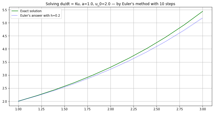
def euler(f, a, b, u_0, n=100):
    """Use Euler's Method to solve du/dt = f(t, u) for t in [a, b], with initial value u(a) = u_0"""
    h = (b-a)/n
    t = np.linspace(a, b, n+1)  # Note: "n" counts steps, so there are n+1 values for t.

    # Only the following two lines will need to change for the systems version
    U = np.empty_like(t)
    U[0] = u_0

    for i in range(n):
        U[i+1] = U[i] + f(t[i], U[i])*h
    return (t, U)
# Demo
if __name__ == "__main__": # Do this if running the .py file directly, but not when importing [from] it.
def f_1(t, u):
"""The simplest "genuine" ODE, (not just integration)
The solution is u(t) = u(t; a, u_0) = u_0 exp(t-a)
"""
return K*u
def u_1(t): return u_0 * np.exp(K*(t-a))
a = 1.
b = 3.
u_0 = 2.
K = 0.5
n = 10
(t, U) = euler(f_1, a, b, u_0, n)
h = (b-a)/n
plt.figure(figsize=[12,6])
plt.title(f"Solving du/dt = Ku, {a=}, {u_0=} — by Euler's method with {n} steps")
plt.plot(t, u_1(t), 'g', label="Exact solution")
plt.plot(t, U, 'b:', label=f"Euler's answer with h={h:0.3}")
plt.legend()
plt.grid(True)
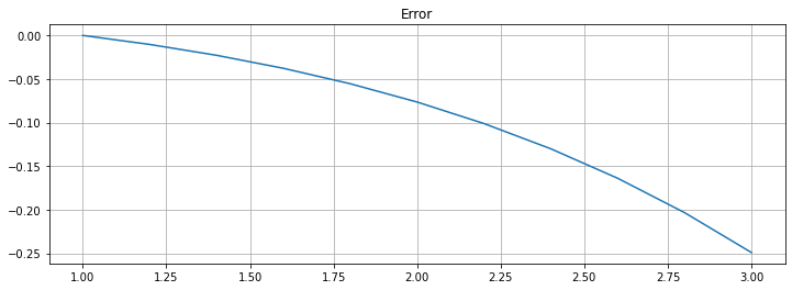
plt.figure(figsize=[12,4])
plt.title(f"Error")
plt.plot(t, U - u_1(t))
plt.grid(True)
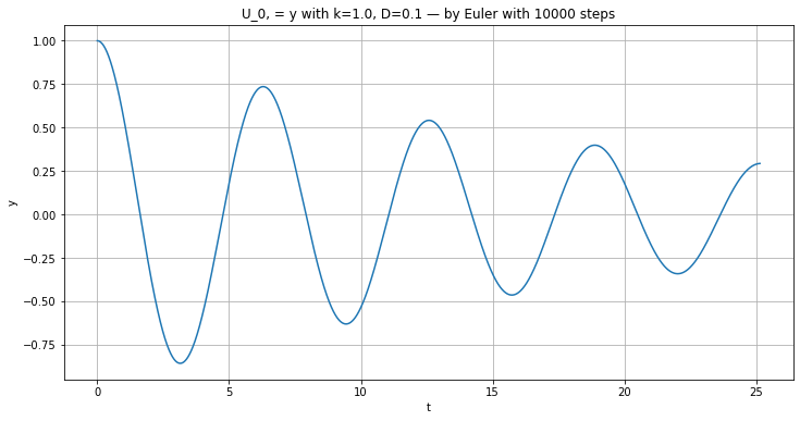
def euler_system(f, a, b, u_0, n=100):
    """Use Euler's Method to solve du/dt = f(t, u) for t in [a, b], with initial value u(a) = u_0
    Modified from function euler to handle systems."""
    h = (b-a)/n
    t = np.linspace(a, b, n+1)  # Note: "n" counts steps, so there are n+1 values for t.

    # Only the following three lines change for the systems version
    n_unknowns = len(u_0)
    U = np.zeros([n+1, n_unknowns])
    U[0] = np.array(u_0)

    for i in range(n):
        U[i+1] = U[i] + f(t[i], U[i])*h
    return (t, U)
# Demo
if __name__ == "__main__": # Do this if running the .py file directly, but not when importing [from] it.
def f(t, u):
return np.array([ u[1], -(k/M)*u[0] - (D/M)*u[1]])
M = 1.0
k = 1.0
D = 0.1
u_0 = [1.0, 0.0]
a = 0.0
b = 8 * np.pi # Four periods
n=10000
(t, U) = euler_system(f, a, b, u_0, n)
y = U[:,0]
Dy = U[:,1]
plt.figure(figsize=[12,6])
plt.title(f"U_0, = y with {k=}, {D=} — by Euler with {n} steps")
plt.plot(t, y)
plt.xlabel('t')
plt.ylabel('y')
plt.grid(True)
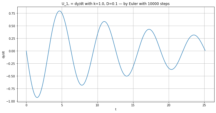
plt.figure(figsize=[12,6])
plt.title(f"U_1, = dy/dt with {k=}, {D=} — by Euler with {n} steps")
plt.plot(t, Dy)
plt.xlabel('t')
plt.ylabel('dy/dt')
plt.grid(True)
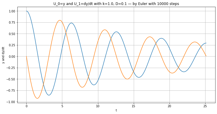
plt.figure(figsize=[12,6])
plt.title(f"U_0=y and U_1=dy/dt with {k=}, {D=} — by Euler with {n} steps")
plt.plot(t, U)
plt.xlabel('t')
plt.ylabel('y and dy/dt')
plt.grid(True)
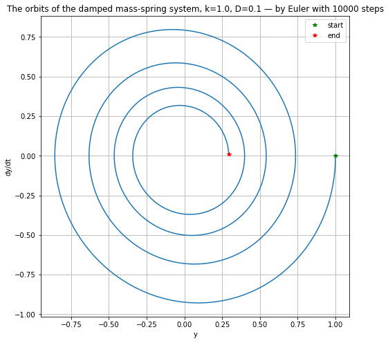
plt.figure(figsize=[8,8]) # Make axes equal length; orbits should be circular or "circular spirals"
if D == 0.:
plt.title(f"The orbits of the undamped mass-spring system, {k=} — by Euler with {n} steps")
else:
plt.title(f"The orbits of the damped mass-spring system, k={k}, D={D} — by Euler with {n} steps")
plt.plot(y, Dy)
plt.xlabel('y')
plt.ylabel('dy/dt')
plt.plot(y[0], Dy[0], "g*", label="start")
plt.plot(y[-1], Dy[-1], "r*", label="end")
plt.legend()
plt.grid(True)
def explicitTrapezoid(f, a, b, u_0, n=100):
    """Use the Explict Trapezoid Method (a.k.a Improved Euler)
    to solve du/dt = f(t, u) for t in [a, b], with initial value u(a) = u_0"""
    h = (b-a)/n
    t = np.linspace(a, b, n+1)  # Note: "n" counts steps, so there are n+1 values for t.

    # Only the following two lines will need to change for the systems version
    U = np.empty_like(t)
    U[0] = u_0

    for i in range(n):
        K_1 = f(t[i], U[i])*h
        K_2 = f(t[i]+h, U[i]+K_1)*h
        U[i+1] = U[i] + (K_1 + K_2)/2.
    return (t, U)
# Demo
if __name__ == "__main__": # Do this if running the .py file directly, but not when importing [from] it.
a = 1.
b = 3.
u_0 = 2.
K = 1.
n = 10
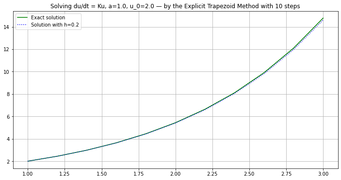
(t, U) = explicitTrapezoid(f_1, a, b, u_0, n)
h = (b-a)/n
plt.figure(figsize=[12,6])
plt.title(f"Solving du/dt = Ku, {a=}, {u_0=} — by the Explicit Trapezoid Method with {n} steps")
plt.plot(t, u_1(t), 'g', label="Exact solution")
plt.plot(t, U, 'b:', label=f"Solution with h={h:0.3}")
plt.legend()
plt.grid(True)
plt.figure(figsize=[12,4])
plt.title(f"Error")
plt.plot(t, U - u_1(t))
plt.grid(True)

# Demo
if __name__ == "__main__": # Do this if running the .py file directly, but not when importing [from] it.
def f_2(t, u):
"""A simple more "generic" test case, with f(t, u) depending on both variables.
The solution for a=0 is u(t) = u(t; 0, u_0) = cos t + (u_0 - 1) e^(-Kt)
The solution in general is u(t) = u(t; a, u_0) = cos t + C e^(-K t), C = (u_0 - cos(a)) exp(K a)
"""
return K*(np.cos(t) - u) - np.sin(t)
def u_2(t): return np.cos(t) + C * np.exp(-K*t)
a = 1.
b = a + 4 * np.pi # Two periods
u_0 = 2.
K = 2.
n = 50
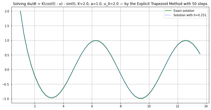
(t, U) = explicitTrapezoid(f_2, a, b, u_0, n)
C = (u_0 - np.cos(a)) * np.exp(K*a)
h = (b-a)/n
plt.figure(figsize=[12,6])
plt.title(f"Solving du/dt = K(cos(t) - u) - sin(t), {K=}, {a=}, {u_0=} — by the Explicit Trapezoid Method with {n} steps")
plt.plot(t, u_2(t), 'g', label="Exact solution")
plt.plot(t, U, 'b:', label=f"Solution with h={h:0.3}")
plt.legend()
plt.grid(True)
plt.figure(figsize=[12,4])
plt.title(f"Error")
plt.plot(t, U - u_2(t))
plt.grid(True)
def explicitMidpoint(f, a, b, u_0, n=100):
    """Use the Explicit Midpoint Method (a.k.a Modified Euler)
    to solve du/dt = f(t, u) for t in [a, b], with initial value u(a) = u_0"""
    h = (b-a)/n
    t = np.linspace(a, b, n+1)  # Note: "n" counts steps, so there are n+1 values for t.

    # Only the following two lines will need to change for the systems version
    U = np.empty_like(t)
    U[0] = u_0

    for i in range(n):
        K_1 = f(t[i], U[i])*h
        K_2 = f(t[i]+h/2, U[i]+K_1/2)*h
        U[i+1] = U[i] + K_2
    return (t, U)
# Demo
if __name__ == "__main__": # Do this if running the .py file directly, but not when importing [from] it.
a = 1.
b = 3.
u_0 = 2.
K = 1.
n = 10
(t, U) = explicitMidpoint(f_1, a, b, u_0, n)
h = (b-a)/n
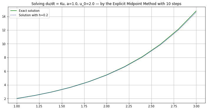
plt.figure(figsize=[12,6])
plt.title(f"Solving du/dt = Ku, {a=}, {u_0=} — by the Explicit Midpoint Method with {n} steps")
plt.plot(t, u_1(t), 'g', label="Exact solution")
plt.plot(t, U, 'b:', label=f"Solution with h={h:0.3}")
plt.legend()
plt.grid(True)
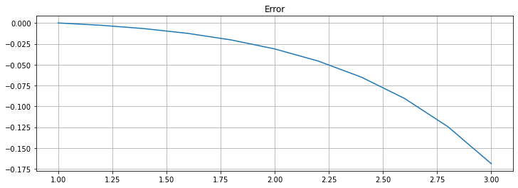
plt.figure(figsize=[12,4])
plt.title(f"Error")
plt.plot(t, U - u_1(t))
plt.grid(True)
# Demo
if __name__ == "__main__": # Do this if running the .py file directly, but not when importing [from] it.
def f_2(t, u):
"""A simple more "generic" test case, with f(t, u) depending on both variables.
The solution for a=0 is u(t) = u(t; 0, u_0) = cos t + (u_0 - 1) e^(-Kt)
The solution in general is u(t) = u(t; a, u_0) = cos t + C e^(-K t), C = (u_0 - cos(a)) exp(K a)
"""
return K*(np.cos(t) - u) - np.sin(t)
def u_2(t): return np.cos(t) + C * np.exp(-K*t)
a = 1.
b = a + 4 * np.pi # Two periods
u_0 = 2.
K = 2.
n = 50
(t, U) = explicitMidpoint(f_2, a, b, u_0, n)
C = (u_0 - np.cos(a)) * np.exp(K*a)
h = (b-a)/n
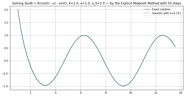
plt.figure(figsize=[12,6])
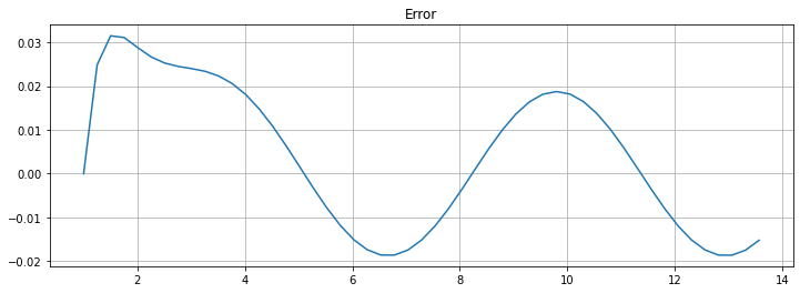
plt.title(f"Solving du/dt = K(cos(t) - u) - sin(t), {K=}, {a=}, {u_0=} — by the Explicit Midpoint Method with {n} steps")
plt.plot(t, u_2(t), 'g', label="Exact solution")
plt.plot(t, U, 'b:', label=f"Solution with h={h:0.3}")
plt.legend()
plt.grid(True)
plt.figure(figsize=[12,4])
plt.title(f"Error")
plt.plot(t, U - u_2(t))
plt.grid(True)
def RungeKutta(f, a, b, u_0, n=100):
    """Use the (classical) Runge-Kutta Method
    to solve du/dt = f(t, u) for t in [a, b], with initial value u(a) = u_0"""
    h = (b-a)/n
    t = np.linspace(a, b, n+1)  # Note: "n" counts steps, so there are n+1 values for t.

    # Only the following two lines will need to change for the systems version
    U = np.empty_like(t)
    U[0] = u_0

    for i in range(n):
        K_1 = f(t[i], U[i])*h
        K_2 = f(t[i]+h/2, U[i]+K_1/2)*h
        K_3 = f(t[i]+h/2, U[i]+K_2/2)*h
        K_4 = f(t[i]+h, U[i]+K_3)*h
        U[i+1] = U[i] + (K_1 + 2*K_2 + 2*K_3 + K_4)/6
    return (t, U)
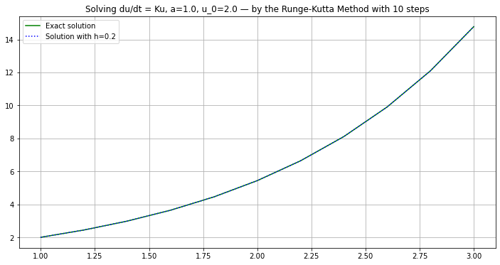
# Demo
if __name__ == "__main__": # Do this if running the .py file directly, but not when importing [from] it.
a = 1.
b = 3.
u_0 = 2.
K = 1.
n = 10
(t, U) = RungeKutta(f_1, a, b, u_0, n)
h = (b-a)/n
plt.figure(figsize=[12,6])
plt.title(f"Solving du/dt = Ku, {a=}, {u_0=} — by the Runge-Kutta Method with {n} steps")
plt.plot(t, u_1(t), 'g', label="Exact solution")
plt.plot(t, U, 'b:', label=f"Solution with h={h:0.3}")
plt.legend()
plt.grid(True)
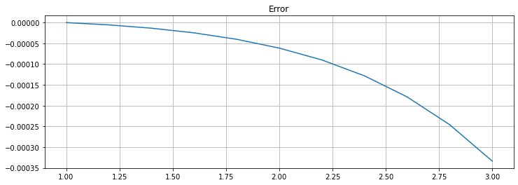
plt.figure(figsize=[12,4])
plt.title(f"Error")
plt.plot(t, U - u_1(t))
plt.grid(True)
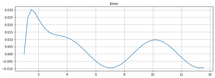
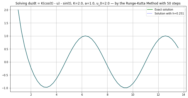
# Demo
if __name__ == "__main__": # Do this if running the .py file directly, but not when importing [from] it.
def f_2(t, u):
"""A simple more "generic" test case, with f(t, u) depending on both variables.
The solution for a=0 is u(t) = u(t; 0, u_0) = cos t + (u_0 - 1) e^(-Kt)
The solution in general is u(t) = u(t; a, u_0) = cos t + C e^(-K t), C = (u_0 - cos(a)) exp(K a)
"""
return K*(np.cos(t) - u) - np.sin(t)
def u_2(t): return np.cos(t) + C * np.exp(-K*t)
a = 1.
b = a + 4 * np.pi # Two periods
u_0 = 2.
K = 2.
n = 50
(t, U) = RungeKutta(f_2, a, b, u_0, n)
C = (u_0 - np.cos(a)) * np.exp(K*a)
h = (b-a)/n
plt.figure(figsize=[12,6])
plt.title(f"Solving du/dt = K(cos(t) - u) - sin(t), {K=}, {a=}, {u_0=} — by the Runge-Kutta Method with {n} steps")
plt.plot(t, u_2(t), 'g', label="Exact solution")
plt.plot(t, U, 'b:', label=f"Solution with h={h:0.3}")
plt.legend()
plt.grid(True)
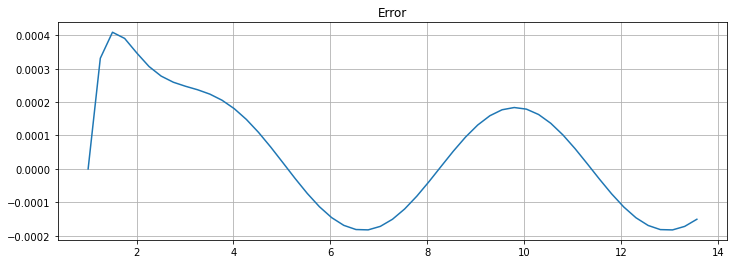
plt.figure(figsize=[12,4])
plt.title(f"Error")
plt.plot(t, U - u_2(t))
plt.grid(True)
def RungeKutta_system(f, a, b, u_0, n=100):
    """Use the (classical) Runge-Kutta Method
    to solve du/dt = f(t, u) for t in [a, b], with initial value u(a) = u_0"""
    h = (b-a)/n
    t = np.linspace(a, b, n+1)  # Note: "n" counts steps, so there are n+1 values for t.

    # Only the following three lines change for the systems version — the same lines as for euler_system and so on.
    n_unknowns = len(u_0)
    U = np.zeros([n+1, n_unknowns])
    U[0] = np.array(u_0)

    for i in range(n):
        K_1 = f(t[i], U[i])*h
        K_2 = f(t[i]+h/2, U[i]+K_1/2)*h
        K_3 = f(t[i]+h/2, U[i]+K_2/2)*h
        K_4 = f(t[i]+h, U[i]+K_3)*h
        U[i+1] = U[i] + (K_1 + 2*K_2 + 2*K_3 + K_4)/6
    return (t, U)
# Demo
if __name__ == "__main__": # Do this if running the .py file directly, but not when importing [from] it.
def f_mass_spring(t, u):
return np.array([ u[1], -(k/M)*u[0] - (D/M)*u[1]])
M = 1.0
k = 1.0
D = 0.1
u_0 = [1.0, 0.0]
a = 0.0
b = 8 * np.pi # Four periods
n = 100 # Should be enough now!
(t, U) = RungeKutta_system(f_mass_spring, a, b, u_0, n)
y = U[:,0]
Dy = U[:,1]
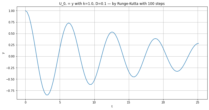
plt.figure(figsize=[12,6])
plt.title(f"U_0, = y with {k=}, {D=} — by Runge-Kutta with {n} steps")
plt.plot(t, y)
plt.xlabel('t')
plt.ylabel('y')
plt.grid(True)
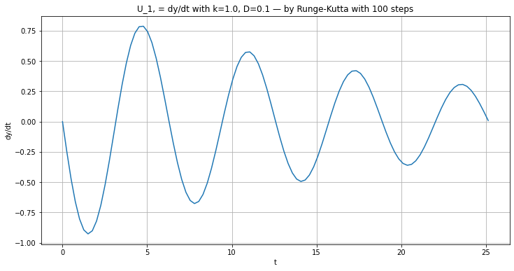
plt.figure(figsize=[12,6])
plt.title(f"U_1, = dy/dt with {k=}, {D=} — by Runge-Kutta with {n} steps")
plt.plot(t, Dy)
plt.xlabel('t')
plt.ylabel('dy/dt')
plt.grid(True)
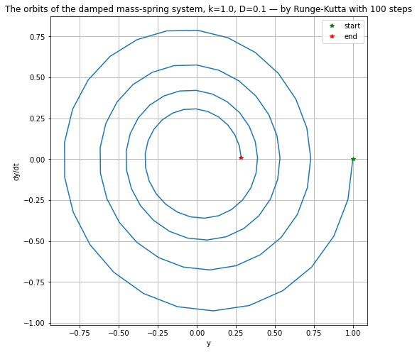
plt.figure(figsize=[8,8]) # Make axes equal length; orbits should be circular or "circular spirals"
if D == 0.:
plt.title(f"The orbits of the undamped mass-spring system, {k=} — by Runge-Kutta with {n} steps")
else:
plt.title(f"The orbits of the damped mass-spring system, k={k}, D={D} — by Runge-Kutta with {n} steps")
plt.plot(y, Dy)
plt.xlabel('y')
plt.ylabel('dy/dt')
plt.plot(y[0], Dy[0], "g*", label="start")
plt.plot(y[-1], Dy[-1], "r*", label="end")
plt.legend()
plt.grid(True)
For the future: an attempt to use the IMPLICIT Midpoint Method
Solving for now with a few fixed point iterations.
def FP_Midpoint_system(f, a, b, u_0, n=100, iterations=1):
    """Use a few iterations of a fixed point method solution of the Implicit Midpoint Method
    to solve du/dt = f(t, u) for t in [a, b], with initial value u(a) = u_0
    Note:
        - the default of iterations=1 gives the Explicit Midpoint Method
        - iterations=0 gives Euler's Method
        """
    h = (b-a)/n
    t = np.linspace(a, b, n+1)  # Note: "n" counts steps, so there are n+1 values for t.

    # Only the following three lines change for the systems version — the same lines as for euler_system and so on.
    n_unknowns = len(u_0)
    U = np.zeros([n+1, n_unknowns])
    U[0] = np.array(u_0)

    for i in range(n):
        K = f(t[i], U[i])*h
        # A few iterations of the fixed point method
        for iteration in range(iterations):
            K = f(t[i]+h/2, U[i]+K/2)*h
        U[i+1] = U[i] + K
    return (t, U)
# Demo
if __name__ == "__main__": # Do this if running the .py file directly, but not when importing [from] it.
def f_mass_spring(t, u):
return np.array([ u[1], -(k/M)*u[0] - (D/M)*u[1]])
M = 1.0
k = 1.0
D = 0.0
u_0 = [1.0, 0.0]
a = 0.0
b = 8 * np.pi # Four periods
n = 200
iterations = 2
(t, U) = FP_Midpoint_system(f_mass_spring, a, b, u_0, n, iterations=1)
y = U[:,0]
Dy = U[:,1]
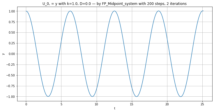
plt.figure(figsize=[12,6])
plt.title(f"U_0, = y with {k=}, {D=} — by FP_Midpoint_system with {n} steps, {iterations} iterations")
plt.plot(t, y)
plt.xlabel('t')
plt.ylabel('y')
plt.grid(True)
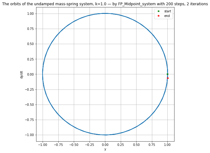
plt.figure(figsize=[8,8]) # Make axes equal length; orbits should be circular or "circular spirals"
if D == 0.:
plt.title(f"The orbits of the undamped mass-spring system, {k=} — by FP_Midpoint_system with {n} steps, {iterations} iterations")
else:
plt.title(f"The orbits of the damped mass-spring system, k={k}, D={D} — by FP_Midpoint_system with {n} steps, {iterations} iterations")
plt.plot(y, Dy)
plt.xlabel('y')
plt.ylabel('dy/dt')
plt.plot(y[0], Dy[0], "g*", label="start")
plt.plot(y[-1], Dy[-1], "r*", label="end")
plt.legend()
plt.grid(True)
This work is licensed under Creative Commons Attribution-ShareAlike 4.0 International