
14. Error Formulas for Polynomial Collocation
Last Revised on Wednesday February 17.
References:
Section 3.2.1 Interpolation error formula of Sauer
Section 3.1 Interpolation and the Lagrange Polynomial of Burden&Faires
Section 4.2 Errors in Polynomial Interpolation of Chenney&Kincaid
14.1. Introduction
When a polynomial \(P_n\) is given by collocation to \(n+1\) points \((x_i, y_i)\), \(y_i = f(x_i)\) on the graph of a function \(f\), one can ask how accurate it is as an approximation of \(f\) at points \(x\) other than the nodes: what is the error \(E(x) = f(x) - P(x)\)?
As is often the case, the result is motivated by considering the simplest “non-trival case”: \(f\) a polynomial of degree one too high for an exact fit, so of degree \(n+1\). The result is also analogous to the familiar error formula for Taylor polynonial approximations.
from numpy import linspace, polyfit, polyval, ones_like
from  matplotlib.pyplot import figure, plot, title, grid, legend
14.2. Error in \(P_n(x)\) collocating a polynomial of degree \(n+1\)
With \(f(x) = c_{n+1} x^{n+1} + c_{n} x^{n} + \cdots + c_0\) a polynomial of degree \(n+1\) and \(P_n(x)\) the unique polynomial of degree at most \(n\) that collocates with it at the \(n+1\) nodes \(x_0, \dots x_n\), the error
is a polynomial of degree \(n+1\) with all its roots known: the nodes \(x_i\). Thus it can be factorized as
On the other hand, the only term of degree \(x^{n+1}\) in \(f(x) - P(x)\) is the leading term of \(f(x)\), \(c_{n+1} x^{n+1}\). Thus \(C = c_{n+1}\).
It will be convenient to note that the order \(n+1\) derivative of \(f\) is the constant \(f^{(n+1)}D^{n+1}f(x) = (n+1)! c_{n+1}\), so the error can be written as
14.3. Error in \(P_n(x)\) collocating a sufficiently differentiable function
Theorem 1. For a function \(f\) with continuous derivative of order \(n+1\) \(D^{n+1}f\), the polynomial \(P_n\) of degree at most \(n\) that fits the points \((x_i, f(x_i))\) \(0 \leq i \leq n\) differs from \(f\) by
for some value of \(\xi_x\) that is amongst the \(n+2\) points \(x_0, \dots x_n\) and \(x\).
In particular, when \(a \leq x_0 < x_1 \cdots < x_n \leq b\) and \(x \in [a,b]\), then also \(\xi_x \in [a, b]\).
Note the similarity to the error formula for the Taylor polynomial \(p_n\) with center \(x_0\):
This is effectively the limit when all the \(x_i_x\) congeal to \(x_0\).
14.4. Error bound with equally spaced nodes is \(O(h^{n+1})\), but …
An important special case is when there is a single parameter \(h\) describing the spacing of the nodes; when they are the equally spaced values \(x_i = a + i h\), \(0 \leq i \leq n\), so that \(x_0 = a\) and \(x_n = b\) with \(h = \displaystyle \frac{b-a}{n}\). Then there is a somewhat more practically usable error bound:
Theorem 2. For \(x \in [a,b]\) and the above equaly spaced nodes in that interval \([a,b]\),
where \(M_{n+1} = \max\limits_{x \in [a,b]} | D^{n+1}f(x)|\).
14.5. Possible failure of convergence
A major practical problem with this error bound is that is does not in general guarantee convergence \(P_n(x) \to f(x)\) as \(n \to \infty\) with fixed interval \([a, b]\), because in some cases \(M_{n+1}\) grows too fast.
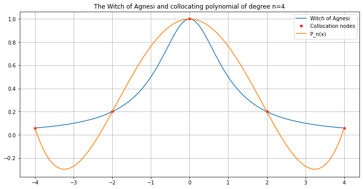
A famous example is the “Witch of Agnesi” (so-called because it was introduced by Maria Agnesi, author of the first textbook on differential and integral calculus).
def agnesi(x):
    """An example sometime know as "the Witch of Agnesi",
    after
    """
    return 1/(1+x**2)
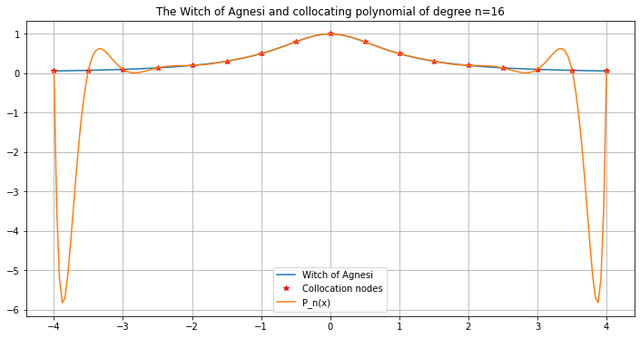
def graph_agnesi_collocation(a, b, n):
figure(figsize=[12, 6])
title(f"The Witch of Agnesi and collocating polynomial of degree {n=}")
x = linspace(a, b, 200) # Plot 200 points instead of the default 50, as some fine detail is needed
agnesi_x = agnesi(x)
plot(x, agnesi_x, label="Witch of Agnesi")
x_nodes = linspace(a, b, n+1)
y_nodes = agnesi(x_nodes)
c = polyfit(x_nodes, y_nodes, n)
P_n = polyval(c, x)
plot(x_nodes, y_nodes, 'r*', label="Collocation nodes")
plot(x, P_n, label="P_n(x)")
legend()
grid(True)
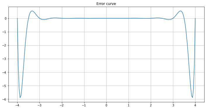
figure(figsize=[12, 6])
title(f"Error curve")
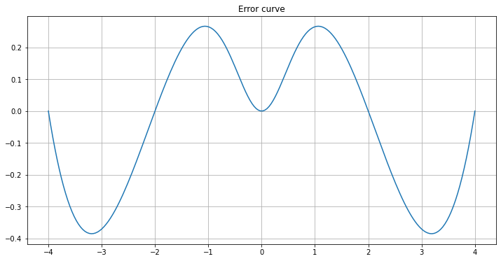
E_n = P_n - agnesi_x
plot(x, E_n)
grid(True)
Start with \(n=4\), which seems somewhat well-behaved:
graph_agnesi_collocation(a=-4, b=4, n=4)
Now increase the number of inervals, doubling each time.
graph_agnesi_collocation(a=-4, b=4, n=8)
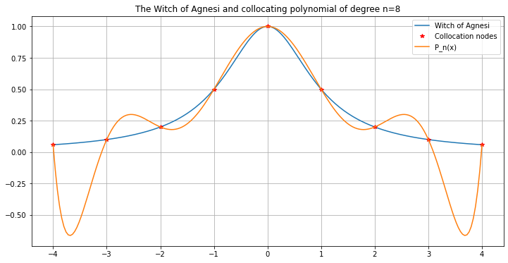
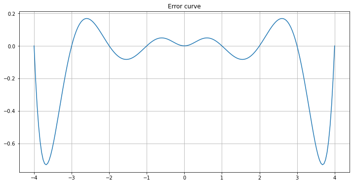
The curve fits better in the central part, but gets worse towards the ends!
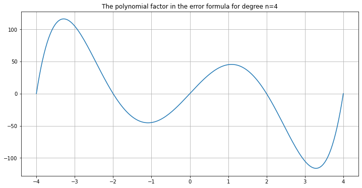
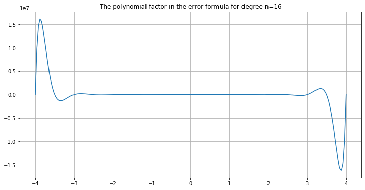
One hint as to why is to plot the polynomial factor in the error formula above:
def graph_error_formula_polynomial(a, b, n):
    figure(figsize=[12, 6])
    title(f"The polynomial factor in the error formula for degree {n=}")
    x = linspace(a, b, 200)  # Plot 200 points instead of the default 50, as some fine detail is needed
    x_nodes = linspace(a, b, n+1)
    polynomial_factor = ones_like(x)
    for x_node in x_nodes:
        polynomial_factor *= (x - x_node)
    plot(x, polynomial_factor)
    grid(True)
graph_error_formula_polynomial(a=-4, b=4, n=4)
graph_error_formula_polynomial(a=-4, b=4, n=8)
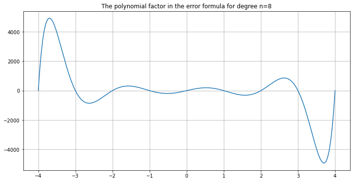
As n increases, it just gets worse:
graph_agnesi_collocation(a=-4, b=4, n=16)
graph_error_formula_polynomial(a=-4, b=4, n=16)
14.6. A Solution: piecewise (linear) interpolation
A solution to this problem is to use collocation with just a fixed number of nodes \(m\) as \(h \to 0\) and the total node count \(n \to \infty\). That is, for each \(x\), approximate \(f(x)\) using just data from a suitable choice of \(m+1\) nodes near \(x\). Then \(M_{m+1}\) is a constant, and one has the convergence result
so long as \(f\) has a continuous derivatives up to order \(m+1\).
But then how does one get an approximation over a fixed interval of interest, \([a, b]\)?
One solution is to use multiple polynomials, by dividing the interval into numerous small ones. The simplest version of this is to divide it into \(n\) sub-intervals of equal width \(h=(b-a)/n\), separated at nodes \(x_i = a + i h\), \(0 \leq i \leq n\), and approximate \(f(x)\) linearly on each sub-inerval by using the two surrounding nodes \(x_i\) and \(x_{i+1}\) determined by having \(x_i \leq x \leq x_{i+1}\): this is piecewise linear interpolation.
This gives the approximating function \(L_n(x)\), and the above error formula, now with \(m=1\) says that the worst absolute error anywhere in the interval \([a, b]\) is
with \(M_2 = \max\limits_{x \in [a,b]} | D^2f(x)|\).
Now clearly, as \(n \to \infty\), the error at each \(x\)-value converges to zero.
14.6.1. Preview: definite integrals (en route to solving differential equations)
Integrating this piecewise linear approximation over interval \([a, b]\) gives the Compound Trapezoid Rule approximation of \(\int_a^b f(x) dx\). As we will soon see, this also has error at worst \(O(h^2), = O(1/n^2)\): each doubling of effort reduces errors by a factor of about four.
Also, you might have heard of Simpson’s Rule for approximating definite integrals (and anyway, you will soon!): that uses piecewise quadratic interpolation and we will see that this improves the errors to \(O(h^4), = O(1/n^4)\): each doubling of effort reduces errors by a factor of about 16.
14.6.2. Aside: computer graphics and smoother approximating curves
Computer graphics often draws graphs from data points this way, most often with either piecewise linear or piecewise cubic (\(m=3\)) approximation.
However, this always gives sharp “corners” at the nodes. That is unavoidable with piecewise linear curves, but for higher degrees there are modifications of this strategy that give smoother curves: piecewise cubics turn out to work very nicely for that.
This work is licensed under Creative Commons Attribution-ShareAlike 4.0 International