15. Random Numbers, Histograms, and a Simulation¶

This work is licensed under Creative Commons Attribution-ShareAlike 4.0 International

15.1. Introduction¶

Random numbers are often useful both for simulation of physical processes and for generating a collection of test cases. Here we will do a mathematical simulation: approximating \(\pi\) on the basis that the unit circle occupies a fraction \(\pi/4\) of the \(2 \times 2\) square enclosing it.

15.1.1. Disclaimer¶

Actually, the best we have available is pseudo-random numbers, generated by algorithms that actually produce a very long but eventually repeating sequence of numbers.

15.2. Module `random` within package `numpy`¶

The pseudo-random number generator we use are provided by package Numpy in its module random – full name numpy.random. This module contains numerous random number generators; here we look at just a few.

We introduce the abbreviation “npr” for this, along with the standard abbreviations “np” for numpy and “plt” for module matplotlib.pyplot witit package `matplotlib

import numpy.random as npr
import numpy as np
import matplotlib.pyplot as plt
%matplotlib inline

15.3. Uniformly distributed real numbers: `numpy.random.rand`¶

First, the function rand (full name numpy.random.rand) generates uniformly-distributed real numbers in the semi-open interval \([0,1)\).

To generate a single value, use it with no argument:

n_samples = 4
for sample in range(n_samples):
    print(npr.rand())

6831120389814106
5548018157238266
8695626004658878
3752686546706374

15.3.1. Arrays of random values¶

To generate an array of values all at once, one can specify how many as the first and only input argument:

pseudorandomnumbers = npr.rand(n_samples)
print(pseudorandomnumbers)

[0.62144348 0.03793401 0.13891253 0.84806369]

However, the first method has an advantage in some situations: neither the whole list of integers from 0 to n_samples - 1 nor the collection of random numbers is stored at any time: instead, just one value at a time is provided, used, and then “forgotten”. This can be beneficial or even essential when a very large number of random values is used; it is not unusual for a simulation to require more random values than the computer’s memory can hold.

15.3.2. Multi-dimensional arrays of random values¶

We can also generate multi-dimensional arrays, by giving the lengths of each dimension as arguments:

numbers2d = npr.rand(2,3)
print('A two-dimensional array of random numbers:\n', numbers2d)
numbers3d = npr.rand(2,3,4)
print('\nA three-dimensional array of random numbers:\n', numbers3d)

A two-dimensional array of random numbers:
 [[0.18395217 0.71429007 0.68437103]
 [0.00242336 0.92888447 0.14129646]]

A three-dimensional array of random numbers:
 [[[0.2511712  0.85518662 0.36048736 0.11214513]
  [0.00948166 0.91241279 0.07428897 0.18599767]
  [0.75078587 0.31421873 0.00762302 0.15589679]]

 [[0.78636402 0.48269234 0.08894184 0.33770037]
  [0.66866924 0.85747635 0.82185659 0.83088524]
  [0.98993293 0.10828591 0.78003614 0.53410965]]]

15.4. Normally distributed real numbers: `numpy.random.randn`¶

The function randn has the same interface, but generates numbers with the standard normal distribution of mean zero, standard deviation one:

print('Ten normally distributed values:\n', npr.randn(20))

Ten normally distributed values:
 [ 1.01125557 -0.51308499  1.47690102 -0.1352893   0.03629515  1.06888055
  0.17867389  0.03297391  1.62309016  0.38036881 -1.45193537 -0.16739935
  1.52999647 -0.24956606  0.62335861 -0.23251452  0.4546426  -0.61267693
  1.24106299  0.52917226]

n_samples = 10**7
normf_samples = npr.randn(n_samples)
mean = sum(normf_samples)/n_samples
print('The mean of these', n_samples, 'samples is', mean)
standard_deviation = np.sqrt(sum(normf_samples**2)/n_samples - mean**2)
print('and their standard deviation is', standard_deviation)

The mean of these 10000000 samples is 0.00032428885458364956
and their standard deviation is 1.0002386370861691

Note The exact mean and standard deviation of the standard normal distribtion are 0 and 1 respectively, so the slight variations above are due to these being only a sample mean and sample standard deviation.

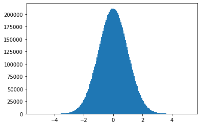
15.5. Histogram plots with `matplotlib.random.hist`¶

matplotlib.random has a function hist(x, bins, ...) for plotting histograms, so we can check what this normal distribution actually looks like.

Input parameter x is the list of values, and when input parameter bins is given an integer value, the data is binned into that many equally wide intervals.

The function hist also returns three values:

n, the number of values in each bin (the bar heights on the histogram)
bins (which I prefer to call bin_edges), the list of values of the edges between the bins
patches, which we can ignore!

It is best to assigned this output to variables; otherwise the numerous values are sprayed over the screen.

# Note: the three output values must be assigned to variables, even though we do not need them here.
(n, bin_edges, patches) = plt.hist(normf_samples, 200)

../_images/random-numbers-and-simulation_17_0.png

15.6. Random integers: `numpy.random.randint`¶

One can generate pseudo-random integers, uniformly distributed between specified lower and upper values.

n_dice = 60
dice_rolls = npr.randint(1, 6+1, n_dice)
print(n_dice, 'random dice rolls:\n', dice_rolls)
# Count each outcome: this needs a list instead of an array:
dice_rolls_list = list(dice_rolls)
for value in (1, 2, 3, 4, 5, 6):
    count = dice_rolls_list.count(value)
    print(value, 'occured', count, 'times')

random dice rolls:
 [4 3 2 3 3 3 3 4 1 6 5 4 4 6 6 3 2 6 5 2 5 4 3 1 4 4 1 1 2 2 3 4 3 4 1 6 1
6 6 6 5 6 6 2 5 6 4 1 3 2 5 4 5 2 3 6 3 3 5]
occured 7 times
occured 8 times
occured 14 times
occured 11 times
occured 8 times
occured 12 times

15.6.1. Specifying bin edges for the histogram¶

This time, it is best to explicitly specify a list of the edges of the bins, by making the second argument bins a list.

With six values, seven edges are needed, and it looks nicest if they are centered on the integers.

bin_edges = [0.5, 1.5, 2.5, 3.5, 4.5, 5.5, 6.5]

(n, bin_edges, patches) = plt.hist(dice_rolls, bin_edges)

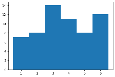
../_images/random-numbers-and-simulation_22_0.png

Run the above several times, redrawing the histogram each time; you should see a lot of variation.

Things average out with more rolls:

n_dice = 10**6
dice_rolls = npr.randint(1, 6+1, n_dice)
# Count each outcome: this needs a list instead of an array:
dice_rolls_list = list(dice_rolls)
for value in (1, 2, 3, 4, 5, 6):
    count = dice_rolls_list.count(value)
    print(value, 'occured a fraction', count/n_dice, 'of the time')
(n, bin_edges, patches) = plt.hist(dice_rolls, bins = bin_edges)

occured a fraction 0.166567 of the time
occured a fraction 0.166454 of the time
occured a fraction 0.166568 of the time
occured a fraction 0.16633 of the time
occured a fraction 0.167526 of the time
occured a fraction 0.166555 of the time

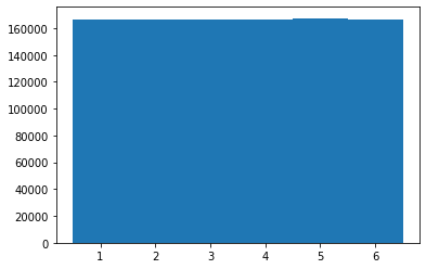
../_images/random-numbers-and-simulation_24_1.png

The histogram is now visually boring, but mathematically more satisfying.

15.6.1.1. Exercise A: approximating \(\pi\)¶

We can compute approximations of \(\pi\) by using the fact that the unit circle occupies a fraction \(\pi/4\) of the circumscribed square:

plt.figure(figsize=[8, 8])
angle = np.linspace(0, 2*np.pi)
# Red circle 
plt.plot(np.cos(angle), np.sin(angle), 'r')
# Blue square
plt.plot([-1,1], [-1,-1], 'b')  # bottom side of square
plt.plot([1,1], [-1,1], 'b')  # right side  of square
plt.plot([1,-1], [1,1], 'b')  # top side of square
plt.plot([-1,-1], [1,-1], 'b')  # left side of square

[<matplotlib.lines.Line2D at 0x7fc7ea44be10>]

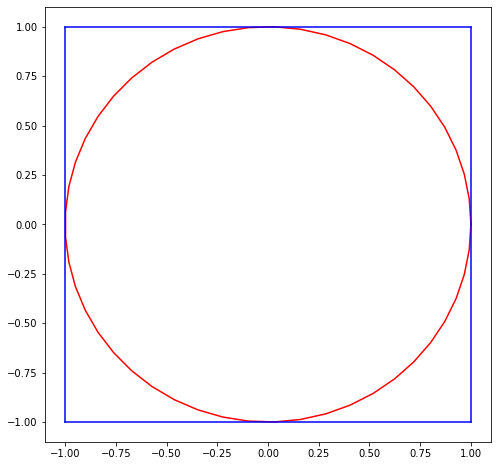
../_images/random-numbers-and-simulation_27_1.png

We can use this fact as follows:

generate a list of \(N\) random points in the square \([-1,1] \times [-1,1]\) that circumscribes the unit circle, by generating successive unifromly distributed random values for both the \(x\) and \(y\) coordinates.
compute the fraction of these that are inside the unit circle, which should be approximately \(\pi/4\). (\(N\) needs to be fairly large; you could try \(N=100\) initially, but will increase it later.)
Multiply by four and there you are!

Do multiple trials with the same number \(N\) of samples, to see the variation as an indication of accuracy.

Collect the various approximations of \(\pi\) in a list, compute the (sample) mean and (sample) standard deviation of the list, and illustrate with a histogram.

15.6.1.2. Exercise B¶

It takes a lot of samples to get decent accuracy, so after part (a) is working, experiment with successively more samples; increase the number \(N\) of samples per trial by big steps, like factors of 100.

For each choice of sample size \(N\), compute the mean and standard deviation, and plot the histogram.

MATH 375. Elementary Numerical Analysis (with Python)