
13. Polynomial Collocation (Interpolation/Extrapolation) and Approximation
Last Revised on Wednesday February 17.
References:
Section 3.1 Data and Interpolating Functions of Sauer
Section 3.1 Interpolation and the Lagrange Polynomial of Burden&Faires
Section 4.1 of Chenney&Kincaid
13.1. Introduction
Numerical methods for dealing with functions require describing them, at least approximately, using a finite list of numbers, and the most basic approach is to approximate by a polynomial. (Other important choices are rational functions and “trigonometric polynomials”: sums of multiples of sines and cosines.) Such polynomials can then be used to aproximate derivatives and integrals.
The simplest idea for approximating \(f(x)\) on domain \([a, b]\) is to start with a finite collection of node values \(x_i \in [a, b]\), \(0 \leq i \leq n\) and then seek a polynomial \(p\) which collocates with \(f\) at those values: \(p(x_i) = f(x_i)\) for \(0 \leq i \leq n\). Actually, we can put the function aside for now, and simply seek a polynomial that passes through a list of points \((x_i, y_i)\); later we will achieve collocation with \(f\) by choosing \(y_i = f(x_i)\).
In fact there are infinitely many such polynomials: given one, add to it any polynomial with zeros at all of the \(n+1\) notes. So to make the problem well-posed, we seek the collocating polynomial of lowest degree.
Theorem Given \(n+1\) distinct values \(x_i\), \(0 \leq i \leq n\), and corresponding \(y\)-values \(y_i\), there is a unique polynomial \(P\) of degree at most \(n\) with \(P(x_i) = y_i\) for \(0 \leq i \leq n\).
(Note: although the degree is typically \(n\), it can be less; as an extreme example, if all \(y_i\) are equal to \(c\), then \(P(x)\) is that constant \(c\).)
Historically there are several methods for finding \(P_n\) and proving its uniqueness, in particular, the divided difference method introduced by Newton and the Lagrange polynomial method. However for our purposes, and for most modern needs, a different method is easiest, and it also introduces a strategy that will be of repeated use later in this course: the Method of Undertermined Coefficients or MUC.
In general, this method starts by assuming that the function wanted is a sum of unknown multiples of a collection of known functions.
Here, \(P(x) = c_n x^n + c_{n-1} x^{n-1} + \cdots+ c_1 x + c_0 = \sum_{j=0}^n c_j x^j\).
(Note: any of the \(c_i\) could be zero, including \(c_n\), in which case the degree is less than \(n\).)
The unknown factors (\(c_0 \cdots c_n\)) are the undetermined coefficients.
Next one states the problem as a system of equations for these undetermined coefficients, and solves them.
Here, we have \(n+1\) conditions to be met:
This is a system if \(n+1\) simultaneous linear equations in \(n+1\) iunknowns, so the question of existence and uniqueness is exactly the question of whether the corresponding matrix is singular, and so is equivalent to the case of all \(y_i = 0\) having only the solution with all \(c_i = 0\).
Back in terms of polynomials, this is the claim that the only polynomial of degree at most \(n\) with zeros \(x_0 \dots x_n\). And this is true, because any non-trivial polynomial with those \(n+1\) distinct roots is of degree at least \(n+1\), so the only “degree n” polynomial fitting this data is \(P(x) \equiv 0\). The theorem is proven.
The proof of this theorem is completely constructive; it gives the only numerical method we need, and which is the one implemented in Numpy through the pair of functions numpy.polyfit and numpy.polyval that we will use in examples.
(Aside: here as in many places, Numpy mimics the names and functionality of corresponding Matlab tools.)
Briefly, the algorithm is this (indexing from 0 !)
Create the \(n+1 \times n+1\) matrix \(V\) with elements
and the \(n+1\)-element column vector \(y\) with elements \(y_i\) as above.
Solve \(V c = y\) for the vector of coefficients \(c_j\) as above.
I use the name \(V\) because this is called the Vandermonde Matrix.
from numpy import array, linspace, polyfit, polyval, zeros_like, empty_like, exp
from  matplotlib.pyplot import figure, plot, title, grid, legend
13.2. Python example with polyfit and polyvalfrom Numpy
As usual, I concoct a first example with known correct answer, by using a polynomial as \(f\).
def f(x):
    return 3*x**4 - 5*x**3 -2*x**2 + 7*x + 4
n = 4
x_nodes = array([1., 2., 7., 5., 4.])  # They do not need to be in order
print(f"The x nodes 'x_i' are {x_nodes}")
y_nodes = empty_like(x_nodes)
for i in range(len(x_nodes)):
    y_nodes[i] = f(x_nodes[i])
print(f"The y values at the nodes are {y_nodes}")
c = polyfit(x_nodes, y_nodes, n)  # Note: n must as be specified; we will see why soon
print(f"The coefficients of P are {c}")
P_values = polyval(c, x_nodes)
print(f"The values of P(x_i) are {P_values}")
The x nodes 'x_i' are [1. 2. 7. 5. 4.]
The y values at the nodes are [   7.   18. 5443. 1239.  448.]
The coefficients of P are [ 3. -5. -2.  7.  4.]
The values of P(x_i) are [   7.   18. 5443. 1239.  448.]
13.2.1. Python presentation aside: pretty-print the result
print("P(x) = ", end="")
for j in range(n-1):  # count up to j=n-2 only, omitting the x and constant terms
    print(f"{c[j]:.4}x^{n-j} + ", end="")
print(f"{c[-2]:.4}x + {c[-1]:.4}")
P(x) = 3.0x^4 + -5.0x^3 + -2.0x^2 + 7.0x + 4.0
13.3. Example 2: \(f(x)\) not a polynomial of degree \(\leq n\)
# Reduce the degree of $P$ to at most 3:
n = 3
# Truncate the data to 4 values:
x_nodes = array([0., 2., 3., 4.])
y_nodes = empty_like(x_nodes)
for i in range(len(x_nodes)):
    y_nodes[i] = f(x_nodes[i])
print(f"n is now {n}, the nodes are now {x_nodes}, with f(x_i) values {y_nodes}")
c = polyfit(x_nodes, y_nodes, n)
print(f"The coefficients of P are now {c}")
print("P(x) = ", end="")
for j in range(n-1):  # count up to j=n-2 only, omitting the x and constant terms
    print(f"{c[j]:.4}x^{n-j} + ", end="")
print(f"{c[-2]:.4}x + {c[-1]:.4}")
P_values = polyval(c, x_nodes)
print(f"The values of P(x_i) are now {P_values}")
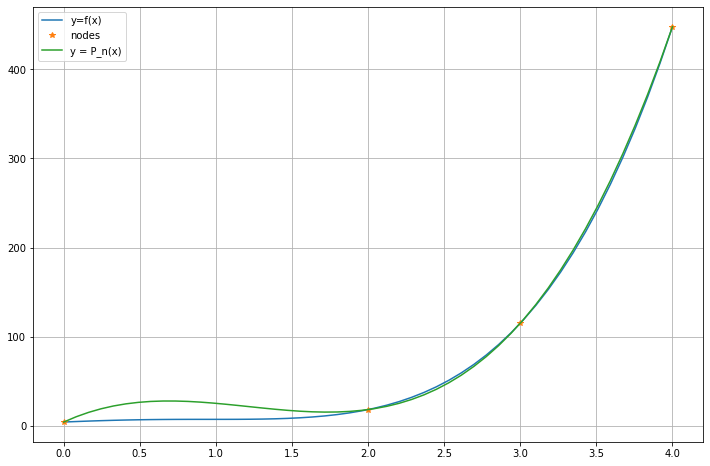
n is now 3, the nodes are now [0. 2. 3. 4.], with f(x_i) values [  4.  18. 115. 448.]
The coefficients of P are now [ 22. -80.  79.   4.]
P(x) = 22.0x^3 + -80.0x^2 + 79.0x + 4.0
The values of P(x_i) are now [  4.  18. 115. 448.]
There are several ways to assess the accuracy of this fit; we start graphically, and later consider the maximum and root-mean-square (RMS) errors.
x = linspace(0, 4) # With a default 50 points, for graphing
figure(figsize=[12,8])
plot(x, f(x), label="y=f(x)")
plot(x_nodes, y_nodes, "*", label="nodes")
P_n_x = polyval(c, x)
plot(x, P_n_x, label="y = P_n(x)")
legend()
grid(True)
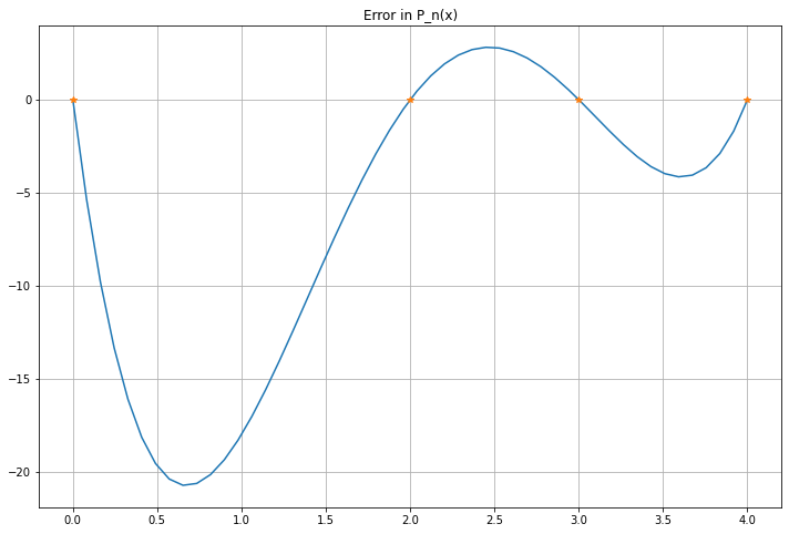
P_error = f(x) - P_n_x
figure(figsize=[12,8])
title("Error in P_n(x)")
plot(x, P_error, label="y=f(x)")
plot(x_nodes, zeros_like(x_nodes), "*")
grid(True)
13.4. Example 3: \(f(x)\) not a polynomial at all
def g(x): return exp(x)
a_g = -1
b_g = 1
n = 3
x_g_nodes = linspace(a_g, b_g, n+1)
y_g_nodes = empty_like(x_g_nodes)
for i in range(len(x_g_nodes)):
    y_g_nodes[i] = g(x_g_nodes[i])
print(f"{n=}")
print(f"node x values {x_g_nodes}")
print(f"node y values {y_g_nodes}")
c_g = polyfit(x_g_nodes, y_g_nodes, n)
print("P(x) = ", end="")

for j in range(n-1):  # count up to j=n-2 only, omitting the x and constant terms
    print(f"{c_g[j]:.4}x^{n-j} + ", end="")
print(f"{c_g[-2]:.4}x + {c_g[-1]:.4}")

P_values = polyval(c_g, x_g_nodes)
print(f"The values of P(x_i) are {P_values}")
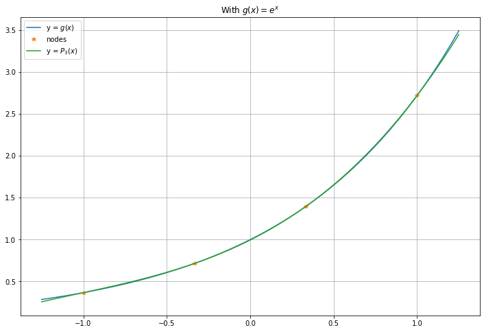
n=3
node x values [-1.         -0.33333333  0.33333333  1.        ]
node y values [0.36787944 0.71653131 1.39561243 2.71828183]
P(x) = 0.1762x^3 + 0.5479x^2 + 0.999x + 0.9952
The values of P(x_i) are [0.36787944 0.71653131 1.39561243 2.71828183]
There are several ways to assess the accuracy of this fit. We start graphically, and later consider the maximum and root-mean-square (RMS) errors.
x_g = linspace(a_g - 0.25, b_g + 0.25) # Go a bit beyond the nodes in each direction
figure(figsize=[12,8])
title("With $g(x) = e^x$")
plot(x_g, g(x_g), label="y = $g(x)$")
plot(x_g_nodes, y_g_nodes, "*", label="nodes")
P_n_x = polyval(c_g, x_g)
plot(x_g, P_n_x, label=f"y = $P_{n}(x)$")
legend()
grid(True)
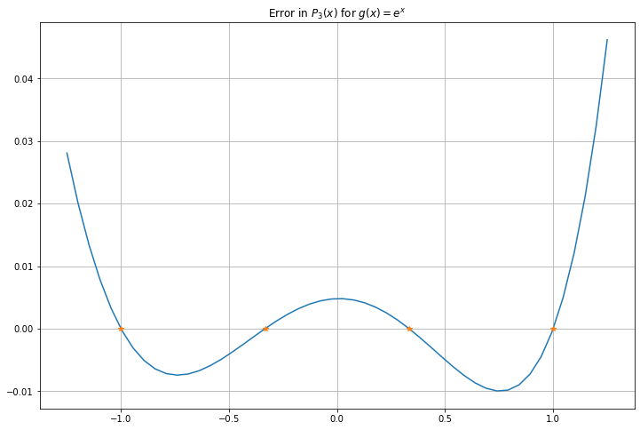
P_error = g(x_g) - P_n_x
figure(figsize=[12,8])
title(f"Error in $P_{n}(x)$ for $g(x) = e^x$")
plot(x_g, P_error)
plot(x_g_nodes, zeros_like(x_g_nodes), "*")
grid(True)
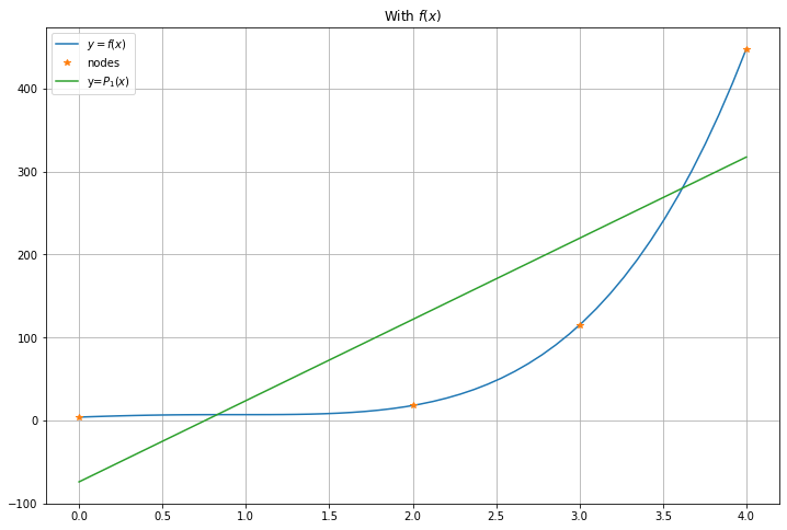
13.5. Why the maximum degree \(n\) must be specified in polyval
The function numpy.polyval can also give a polynomial of lower degree, in which case it is no longer an exact fit; we will consider this next;
returning to the first example of the quartic \(y = f(x)\).
m = 1  # m is the maximum degree of the polynomial: m < n now
c_m = polyfit(x_nodes, y_nodes, m)
print(f"The coefficients of P are {c_m}")

P_m_x = polyval(c_m, x)

# Try to print P(x) again:
print(f"P_{m}(x) = ", end="")
for j in range(m-1):
    print(f"{c_m[j]:.4}x^{m-j} + ", end="")
print(f"{c_m[-2]:.4}x + {c_m[-1]:.4}")
print(f"The values of P(x_i) are {P_values}")

figure(figsize=[12,8])
title("With $f(x)$")
plot(x, f(x), label="$y=f(x)$")
plot(x_nodes, y_nodes, "*", label="nodes")
plot(x, P_m_x, label=f"y=$P_{m}(x)$")
legend()
grid(True)
The coefficients of P are [ 97.91428571 -74.05714286]
P_1(x) = 97.91x + -74.06
The values of P(x_i) are [0.36787944 0.71653131 1.39561243 2.71828183]
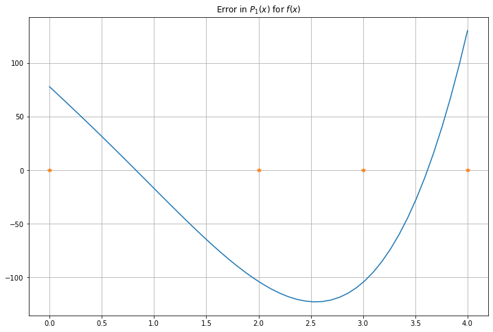
P_error = f(x) - P_m_x
figure(figsize=[12,8])
title("Error in $P_1(x)$ for $f(x)$")
plot(x, P_error, label="y=f(x)")
plot(x_nodes, zeros_like(x_nodes), "*")
grid(True)
13.6. What is the degree \(m\) polynomial given by polyfit(x, y, m)? Least squares fitting.
Another form of polynomial approximation is to find the polynomial of degree at most \(m\) that gives the “best fit” to more data: \(n > m\) points. Then one cannot demand zero error at each point, and so instead aim to minimize some oveall measure of error.
Given a function \(P(x)\) intended to approximately fit a set of data points \((x_i, y_i)\), the approximation errors are the values \(E_i = y_i - P(x_i)\) at each node. Considerening these as forming a vector \(e\), two error minimization strategies are most often used:
Minimize the worst case error, by mimimizing the largest of the absolute errors \(|E_i|\) — this is choosing \(P\) to minimize \(\| E \|_\infty\), often called Chebychev approximation.
Minimize the average error in the root-mean-square sense — this is minimizing the Euclidean norm \(\| E \|_2\).
This time, the Euclidean norm or RMS error method is by far the easiest, giving a simple linear algebra solution.
For now, a quick sketch of the method; the justification will come soon.
If above we seek a polynomial of degree at most \(m\) with \(m \leq n\), we still get a system of equations \(V c = y\), but now \(V\) is \((n+1) \times (m+1)\), \(c\) is \(m+1\) and \(y\) is \(n+1\), so the system is overdetermined.
At this point the “+1” bits are annoying, so we will change notation and consider a more general setting:
Given a \(n \times m\) matrix \(A\), \(n \geq m\), and an \(n\)-vector \(b\), seek the \(m\)-vector \(x\) that is the best approximate solution of \(Ax = b\) in the sense that the residual \(Ax - b\) is as small as possible. It turns out that the solution comes from multiplying through by \(A^T\), getting
which is now an \(m \times m\) system of equations with a unique solution — and it is the “right” one!
This work is licensed under Creative Commons Attribution-ShareAlike 4.0 International